Using Numerical Simulations in Intermediate Macroeconomics

This case study presents, discusses, and reflects on the use of numerical simulations, in particular using Excel, in a second year Macroeconomics unit at the University of Manchester, part of a B.Sc. in Economics.

Background

One of the most common critiques to Macroeconomics teaching is that students struggle to see the connection between the theoretical models and reality. Theoretical models are usually presented in an oversimplified and abstract way, most of the time resorting to extreme aggregation or representative agents, which does not resonate easily with reality. One easy example to mention is the concept of the aggregate production function. Moreover, a lot of time is dedicated to the mathematics of those models, showing all the steps to derive the equilibrium solution and analysing the effects of a shock in the solution of the model, algebraically and/or graphically.

To mitigate such critique and to make Macroeconomics more digestible for students, it is common to bring real life examples to teaching, such as news articles, case studies or even simply using easily available macroeconomic data. Although using macroeconomic data can be really powerful, I find that the jump from the theory to the empirics is sometimes too big. Therefore, solving macroeconomic models by numerical simulations rather than algebraically can reduce the gap between the theory and the data. In addition, using numerical simulations to find and visualize the model's solutions and dynamics in real time can promote students' engagement, active learning and addresses additional digital literacy skills, such as Excel skills. A few important things are worth to clarify from the starting point.

First, numerical simulations here mean assuming numerical values to the model's parameters and initial values (if it is a dynamic model) and using the computer to solve the model's equations for that set of numbers. Any relevant software can be used for that, from the most simple and generic to the most advanced and specific ones, depending on the knowledge of the students and the skillset you want them to develop. One could use any software to implement such practice, but we opted to use the simplest and most generic one, Excel, since it was the first time this approach was implemented in the unit. However, there have been some experiences with specifically designed programs or online platforms (for instance, Rolesia and Econland) and other generic software as well, such as Matlab and R (see, for instance, https://macrosimulation.org/). Excel has another advantage in comparison with specific designed platforms: although the latter can be more interactive and visually appealing, Excel allows a better transparency and manipulation of the mechanics behind the simulations. It is also worth mentioning that the aesthetics of the Excel spreadsheet can be improved.

Second, solving macroeconomic models by numerical simulation is not a substitute for the algebraic solution and analysis. It does not replace the presentation and discussion of the model's equation in abstract form. In fact, I argue that for most macroeconomic models (excluding those that do not have analytical solution by construction, but this is not the case in most intermediate macroeconomic models), a good analytical understanding is crucial and necessary for the numerical solution. After all, the computer is solving the model for a given set of numbers based on the analytical equations of the model, and they must be given to the software correctly. Students must understand well the equations in the background of the numeric simulations.

The rest of the case study will focus on one example, the Solow Growth Model, for its simplicity (there are many other similar tools specifically on the Solow Growth Model, such as https://shiny.demog.berkeley.edu/josh/solow_2017/ , https://demonstrations.wolfram.com/SimpleSolowModel/ and https://www.youtube.com/watch?v=n7b574aE5BE , the last one being very similar to the approach described in this case study), but the same approach has been implemented for other models in the unit, such as the two-period consumption model, a simple dynamic general equilibrium model and a Keynesian stock-flow consistent model (a similar approach is reported for a Dynamic General Equilibrium model by Bongers et. al. (2020))

Using numerical simulations during the lecture

Students are presented to the Solow Growth Model as the baseline conventional macroeconomic model to explain the process of economic growth, its determinants, and the convergence or not between two countries. In the first part of the lecture, they are presented with and discuss some stylized facts on growth, the model's assumptions and its equations.

1. Y = z(K^αN^1−α)
2. C = (1 − s)Y
3. K′ = K(1 − d) + I
4. N′ = (1 + n)N

It can be easily shown that, under competitive equilibrium (Y = C + I), if α < 1, there is a steady state level of income per worker (Y/N) to which the economy will converge. The steady state can be derived and demonstrated algebraically and graphically like below:

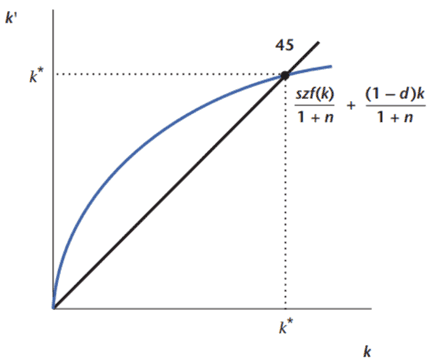
Source: Williamson (2018)

Deriving the result algebraically would take a good number of minutes in the lecture and would be mainly mathematical steps. Full derivations can easily be found in most macroeconomic textbooks and can be given asynchronously in notes or videos. Moreover, this traditional exposition makes evident the lack of connection to real world, as the solution is given purely in an abstract form, where even the passage of time is not quite clear, the same point argued by DeLong (2020). Finally, some shock dynamics, such as a change in the savings rate, are analyzed but in the same traditional manner using comparative statics. The second half of the lecture, though, moves into the numerical simulation. Notice that, even though all the mathematical steps to the solution were not presented in detail, this initial part is necessary for the numerical simulations, to establish the model's equations and discuss the economic mechanism in a general, theoretical, way.

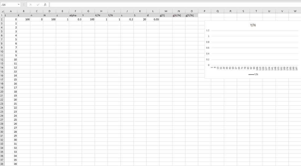
Students are then given an incomplete Excel spreadsheet, henceforth the Simulator. They have access to it already in the VLE and they can open it on their own device simultaneously with the lecture exposition. It has one column for each of the model's parameters and variables and each row is a time period. The use of discrete time periods is quite facilitating as students can easily understand it as one year or one quarter, for instance (the theoretical debate in macroeconomics around the use of continuous or discrete time is much more complex and outside the scope of the case study, though). Finally, one diagram is already pre-defined, although it is blank since the values are still missing:

Click to enlarge

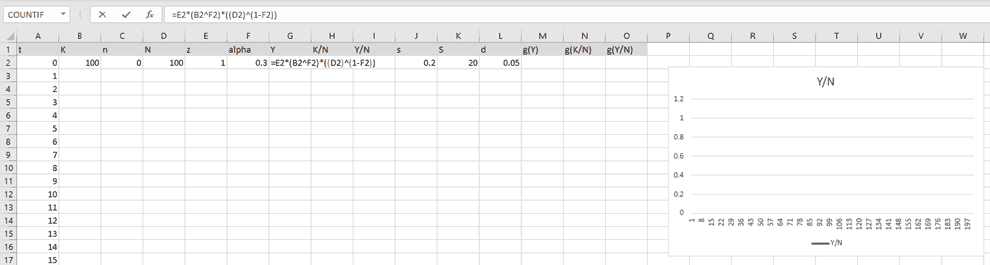
One can see that some parameter and variable initial values are already pre-defined. These are defined arbitrarily. To promote students' engagement, I usually asked them to suggest other values during the lecture. Moreover, they could potentially use empirical data to find appropriate values to calibrate the model for a specific country, for instance. We did this superficially during tutorials, after the model and the simulator were presented in the lecture. The calculation of the model's key variables is shown and discussed. Here, for instance, the output is calculated as in equation 1 above.

Click to enlarge

A few other calculations are still needed, for instance the future capital stock and the future population. This is done together with the students to test their understanding given the first part of the lecture. Then, everything can be calculated for time period 1.

Click to enlarge

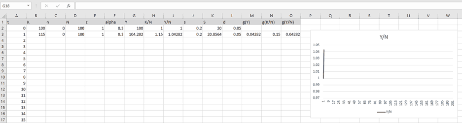
Now, with period 1 values, period 2 can be calculated in the exact same manner. In fact, as the calculations are the same for every period, the functions can easily be extended in Excel for any number of periods.

Click to enlarge

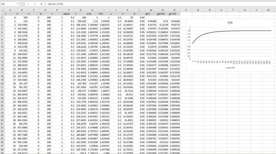
In real time, students obtain simulated values for all the macroeconomic variables in the Solow Growth model for several periods in time. They can observe the values for a single period if they wish and they can check visually and numerically if this economy reaches the steady state or not, or how long it takes to reach the steady state for that set of values. The diagram for income per capita is created instantaneously and students can create other plots for other variables as well, developing their Excel skills. The can now “play” with different initial values and parameters and see how the model yields different results. Simple shocks, such as the previously mentioned change in the savings rate, can be implemented, in or out of the steady state, like below:

Click to enlarge

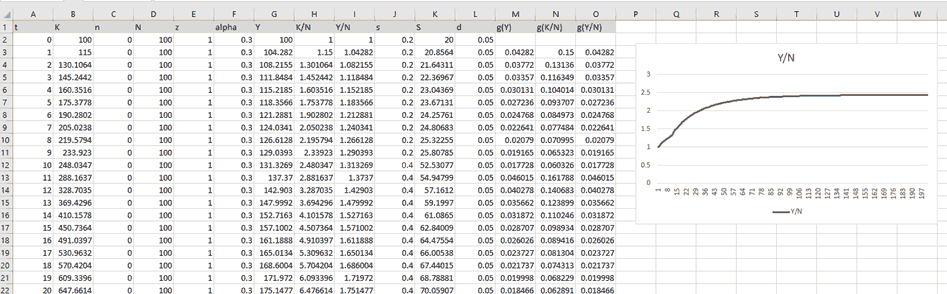
A final exercise is then done between students. Pairing up, each can choose an initial value of the stock of capital, keeping everything else the same for both, and check if “their countries” will converge or not to the same level of capital per capita even with initial different levels (Spoiler: they will converge if everything else is the same).

Assessments

To assess their understanding on the use of the simulator and the model itself, we can give them a set of values and ask them to find and report the obtained value for a specific variable in a specific time period, for instance. There are two main advantages of assessing that way: (1) answers are very specific and cannot be easily be obtained in online search mechanisms, previous exams or even artificial intelligence models, as it requires the student's individual grasp and practice on the use of the simulator; (2) value set can be easily randomized for each student and even the asked variable and time period can be randomized, potentially mitigating some collusion.

Moreover, their modelling skills themselves can be tested as we can also ask students to change or adapt the simulators for a given new equation or theorem. In fact, this is what we asked students to do in the below example, as they needed to extend the established Solow model to account for Human Capital therefore changing the existing simulator they have available. We used the Mobius platform to implement and randomize such questions, as shown above, although there might be other possible ways to do it:

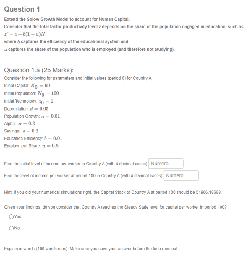
There are also some other things to take into account in that approach. This cannot be the only type of question in the assessment, as it does not access the student's understanding of the economic mechanisms and logic behind the model. In fact, I combined such questions with open written questions in which the student needs to explain, using only words, the economic mechanisms and effects behind the values they find.

Finally, as it can be seen in the illustrative example above, more advanced skills can be tested, such as problem-solving skills, building up the foundation for advanced model-building skills required in Macroeconomics. In this question, the students had to extend the baseline Solow Growth model, adding a new theoretical element that is given only abstractly. They should be able to translate the theory in its abstract level and implement it in the simulator they already have. Only then they would be able to find the answers.

Feedback

The overall feedback from the students was positive. By actively doing practical things to understand and visualize a macroeconomic model during the lecture, students showed more engagements, perceived in relatively high lecture attendance throughout the course and active participation in the lecture with questions and suggestions.

Here are some qualitative comments from students:

• “The use of diagrams and theory first then practical approach was really good and helped in gaining a clearer understanding”
• “We were taught how to the macro concepts operate in real life scenarios by looking at spreadsheets.”
• “I think the Excel walkthroughs were interesting and definitely a relevant and transferable skill that made the module different.”

Here are some comments from a Senior Peer Reviewer:

“First, Matheus presented the elements of the model; he then referred to an online spreadsheet containing a representation of the model, populated cells with values to illustrate the effect of one part on another, asking students questions as he went along. When the model was fully populated, he cleverly modelled the effects of multiple iterations, producing an effective visualisation of the resulting cycles. I thought this was effective teaching with good attempts at involving the students in a very technical exercise.”

Conclusions

• Numerical simulations are an alternative way to present, solve, analyse and discuss macroeconomic models. They complement purely analytical and theoretical exposition, creating a bridge between models and empirical data for students.
• Numerical simulations are an opportunity to promote digital literacy skills, such as the use of key software like Excel and R, in the context of macroeconomics. In a slightly more advanced context, they can also be an opportunity to promote problem-solving skills.
• Numerical simulations, if used during the lecture delivery, can promote students' engagement, as they can actively work independently and they can find and visualize the model's solution in real time. Simulation also promotes creativity and exploration, as students are encouraged to “play” with different set of values.
• Numerical simulations can be used as a form of assessment. Their main advantage is the potential mitigation of collusion as sets of values can be easily randomized for different students. In a slightly more advanced way, the student's ability to translate analytical equations to numerical simulations itself can be assessed, testing their problem-solving skills and building the foundations for advanced model-building skills.
• The overall feedback from the students was positive. They showed more interest and engagement during the lectures and valued the less abstract way to present macroeconomics.

References

Bongers, A., Gómez, T. and Torres, J. L., 2020. Teaching dynamic general equilibrium macroeconomics to undergraduates using a spreadsheet. International Review of Economics Education, 35, p. 100197. https://doi.org/10.1016/j.iree.2020.100197

DeLong, B., 2020. Simulating the Solow Growth Model https://delong.typepad.com/teaching_economics/simulating-solow.html

Williamson, S. D., 2018. Macroeconomics, 6th Edition, Global Edition. Pearson Education Limited, UK OCLC 1017001536

Guest, J., 2015. Reflections on ten years of using economics games and experiments in teaching. Cogent Economics & Finance, 3(1), p. 1115619. https://doi.org/10.1080/23322039.2015.1115619

Becker, W. E., 2000. Teaching economics in the 21st century. Journal of Economic Perspectives, 14(1), pp. 109-119. https://doi.org/10.1257/jep.14.1.109

Colander, D., 2004. The art of teaching economics. International Review of Economics Education, 3(1), pp. 63-76. https://doi.org/10.1016/S1477-3880(15)30144-4

Chulkov, D. and Wang, X., 2020. The Educational Value of Simulation as a Teaching Strategy in a Finance Course. e-Journal of Business Education and Scholarship of Teaching, 14(1), pp. 40-56.

Youngberg, D., 2019. Video games in teaching economics. Teaching Economics: Perspectives on Innovative Economics Education, pp. 9-31. https://doi.org/10.1007/978-3-030-20696-3_2