Case 3: The hold-up problem (computerised)

The hold-up problem is central to the theory of incomplete contracts. It shows how the difficulty in writing complete contracts and the resulting need to renegotiate can lead to underinvestment. We describe here the design of a simple teaching experiment that illustrates the hold-up problem. The model used is a simple perfect information game. The experiment can hence also be used to illustrate the concept of subgame perfect equilibrium and the problem of making binding commitments. In contrast to other perfect information games like the ultimatum or the trust game, the backward induction solution predicts well in our experiment. It is hence a good experiment to conduct in order to illustrate game theory before models where fairness considerations are discussed.

The hold-up problem (see Hart, 1995) results from situations where it is difficult to write complete contracts. When one party has made a prior commitment to a relationship with another party, the latter can ‘hold up’ the former for the value of that commitment. It is argued that the possibility of hold-up can lead to underinvestment in relationship-specific investments and hence to inefficiency. An often quoted (but also sharply disputed) historic example concerned the US car industry. Fisher Body had an exclusive contract to supply body parts for the cars of General Motors. They were the only ones who could deliver the parts according to the specifications needed by GM. In the 1920s there was a sharp increase in demand that exceeded all expectations that were held at the time when the contract was written. It is claimed that Fisher Body used this unforeseen development to hold up General Motors, amongst others, by increasing the price for the additional parts produced.

In our highly stylised game there are two players, the Buyer (aka GM) and the Supplier (aka Fisher Body). In a first stage, the Buyer makes a relationship-specific investment (i.e. decides to set up their line of production such that it depends on specific car body parts delivered by Fisher Body). Then (due to the unforeseen increased demand), the Supplier has the opportunity to raise the price (for the additional demand). In case the price is raised, the Buyer can, at their loss, change the Supplier.

We run two treatments of this game which differ only by one parameter. We sketch here the computerised version available via our FEELE website. More details, and a hand run version, are discussed in (Balkenborg, Kaplan and Miller, 2009a, b). In both treatments it is optimal for the Supplier to hold up the Buyer and for the Buyer to accept the hold-up. In the first treatment it is optimal to invest even if there is a hold-up while in the second treatment it is better not to invest due to the hold-up. We choose this set-up because it allows students first to learn that there will be a hold-up and then to experience the economic consequence of underinvestment caused by the hold-up problem. We tend to run 8–10 rounds of each treatment with a different random pairing for each round. An even number of players is needed.

The first game is given in game tree form in the following graph.

Part 1 Payoffs: (Buyer, Supplier)

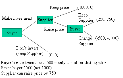
If no investment is made, both players get zero. The investment costs 500 and the gross value produced is 1500. In the initial contract all surplus goes to the Buyer and they get 1000 while the Supplier makes zero profit. The Supplier can hold up the Buyer by raising their price by 750 and leaving the Buyer with 250. The Buyer could change the Supplier, but this hurts everybody. The Buyer loses their investment and the Supplier loses all their business with the Buyer.

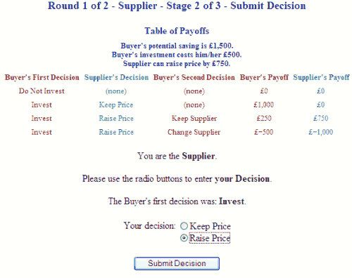
Once the number of players is determined, we can complete the set-up of the experiment and give the students the access code to log in to the experiment via our website. They are then assigned the roles of Buyers and Suppliers and can work through the computerised instructions. In each period the program randomly matches Buyers and Suppliers. Sequentially the game is then played, with first the Buyer deciding whether to invest, followed, if applicable, by the Supplier’s decision whether to raise the price and the Buyer’s decision whether to change the Supplier

In the following screenshot the Supplier is asked to keep or raise their price. The design of the screen is very simple to keep the emphasis on the basic decision.

Typically subjects learn quickly to play the backward induction equilibrium. This means that the Buyer learns that their threat to change the Supplier is ineffective because it is too costly, and therefore the Buyer is held up, i.e. the price is raised. It still pays for the Buyer to make the investment.

This changes in the second treatment. The only number we alter is the cost of the investment which is raised to 1000. As a consequence, the Buyer loses from the investment if they are held up. The payoffs are now illustrated in the following game tree.

Part 2 Payoffs: (Buyer, Supplier)

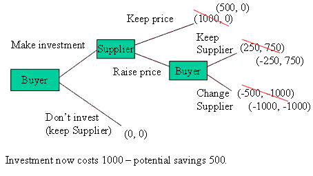
In part 2 of the game the Suppliers are typically held up when possible, and the investment is made much less often.

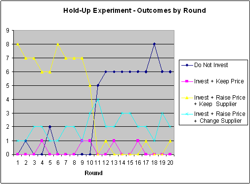
The next figure shows how often each possible outcome arose in the experiment.

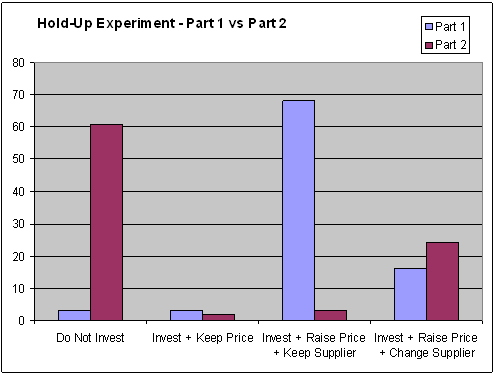
Notice that there is a minority of Buyers who switch Supplier after the price has been raised. (This did not happen in all the sessions we ran.) The rationality of these Buyers is an important point for class discussion: what were they trying to achieve?

The second figure shows the development from period to period.