A pedagogically-driven approach to teaching higher-powered unit root testing
Summary
“Mandatory numbers oblivion!”. Might this be a standard student response to econometrics instruction appearing inaccessible and abstract? Could the study of econometrics in such circumstances only be regarded as a ‘necessary evil’, with students merely recognising it as a mechanism to evidence their marketable quantitative skills? Clearly such gloomy outlook can, and should be, avoided. This is characteristically achieved by adopting a ‘hands-on’ approach, ensuring that econometrics is paramount to the student’s active learning experience. Under such a framework, econometrics becomes aspirational and provides an energetic environment in which relevance and purpose are apparent.
This paper, by pursuing complementary simulation-based and research-driven empirical analyses, provides a case study into the teaching of ‘higher-powered unit root testing’. A familiar component of higher-level econometric provision, the algebraic and technical components of this topic provide a fertile ground to eliminate the ‘necessary evil’ perception of econometrics. If delivery is based upon the melding of a textbook-supported lecture with a ‘plug-and-play’ workshop, it could provide a picture-perfect illustration of how to disengage. However, adopting a pedagogically-inspired approach, this can be averted.
This pedagogy includes standard issues, such as awareness of the literature into the development of transferable and employability-related skills. However, other elements may prove to be less familiar and more nuanced in their nature. For example, we stress how delivery should be shaped on an awareness of: effective active learning strategies; the distinction between behavioural and cognitive activities; and ‘guided’ or ‘discovery-led’ learning approaches. This exemplifies our view that the econometrician should always seek to transform and go beyond stock higher-education soundbites. For example, we argue that the ‘tick-box’ application of ‘research-led’ teaching should be circumvented. Rather than just providing passive observation of someone’s published research, we contend that students should be immersed in the process and directly undertake research-related activities. Thus, by embedding clearly identified pedagogical objectives in the process, a ‘research-driven’ framework can be derived which emphasises the relevance and purpose of econometrics.
1. Econometrics is more than technical
Unit root testing will be all too familiar for anyone involved in the instruction of upper-level econometrics modules. Classroom coverage will typically commence with consideration of the seminal Dickey-Fuller (DF) test (Dickey-Fuller, 1979). Discussion of the power of this test naturally leads to consideration of the GLS-based DF (DF-GLS) test (Elliott et al., 1996). While Müller and Elliott (2003) note that there is no uniformly most powerful unit root test, the GLS-based DF test has gained prominence in the research literature as a higher-powered alternative to the DF test.
When considering the delivery of material on the DF-GLS test within the classroom, it is possible that an instructor might get stuck in the doldrums of mechanical detail. Undoubtedly there is a myriad of ‘technicalities’ to be considered when presenting the DF-GLS test: the application of quasi-differencing; the use of deterministics despite their absence from the test equation employed; the need for a prior regression before reaching the testing equation of interest; consideration of non-standard distributions which vary according to whether an ‘intercept’ or ‘trend’ model specification is considered; and the utilisation of finite-sample distributions.
Such detail threatens a perception of obscurity. The lecturer may appear powerless in avoiding exasperating abstract detail. Engagement levels could flitter away, with that lecturer stuck on presenting a stream of monotonous algebra. This is a mindset that should be alien to the modern econometrician. The discipline should be seen for its splendour: while it is technical, it is also immersed in practicality. It is through consideration of both traits that instruction can flourish. While the technical nature of the discipline provides concrete foundations to upon which to build delivery and assessment, its practical nature allows pedagogical developments to be drawn upon to shape their design. Consequently, passive observation is avoided.
Each year the learning and teaching gurus will offer a barrage of pedagogical demands for instructors to embrace: calls to promote student engagement; training in the utilisation of active learning methods; mechanisms to modernise through the incorporation of research; and continuous adaptation to develop transferable skills. Cohesion across these demands is offered through one decisive word, ‘doing’: ‘doing’ rather than listening supports engagement; active learning involves ‘doing’; research is what academics are ‘doing’; and transferable skills concern the development of an ability to ‘do’. More specifically, the practical nature of econometrics promotes: genuine inclusion of research where the learner themself is ‘doing’, rather than simply viewing the activities of another; and the development of data manipulation and coding skills to independently support employability. However, econometrics can go a step further to ensure that the form of ‘doing’ addresses the important distinction between learning-by-doing and learning-by-thinking (Mayer, 2004, p.17). Here, the significant issue is that students are not just active, but active in a manner that requires cognitive activities linked to higher-order skills (such as the transferral or application of acquired knowledge).
Our overall objective is to stimulate the instruction of higher-powered unit root testing under the lens of these pedagogical interests. To tease out intricacies, we concurrently use simulation and research-driven empirical analyses. The simulation analysis deepens understanding by challenging participants to develop knowledge of the structure of the DF-GLS test ahead of its subsequent transferral to a coding arena. Such synthesis of alternative forms of information is consistent with the cognitive, rather than simply behavioural, activity necessary to develop effective active learning (Mayer, 2004, 2021). As will be documented later, the simulation analysis involves the creation of results which encompass both the distributional properties of the test and also its empirical application. While the ‘distributional’ element assists insight into inference, finite-sample distributions, critical values and p-values, an empirical element arises through a ‘reproduction’ component in which the automated findings of software are duplicated.
As has been noted previously (see Cook and Watson, 2023a), the use of replication or reproduction exercises has many benefits, including: the development of self-efficacy (Bandura, 1977; Zahaciva et al., 2005) and the addressing of anxiety towards quantitative methods (Dreger and Aiken, 1957; Dowker et al., 2016). The research-related empirical element involves appreciation of topical research using real-world data. It necessitates ‘doing’ which challenges comprehension of the appropriate empirical application, the drawing of inferences and relating personal results to those in the published empirical literature. This reveals the true motivation of the econometrics instructor: namely, to derive information on topics of interest. For the research issue chosen here, that refers to the characteristics of house price diffusion. Specifically, can the DF-GLS test provide evidence in support of the ripple effect hypothesis?
To achieve our objectives, this paper first builds from consideration of the DF-GLS test. Here we provide the needed background information that supports the later cognitive processing required for effective active learning. We then shift attention to our simulation and research goals. The simulation analysis, presented in Section 3, includes code to support the generation of critical values for the DF-GLS test in both its intercept and trend model forms. Using the flexibility afforded by this code to allow individual tailoring, it is possible to vary the extent to which ‘discovery’ and ‘guided’ learning are utilised (Mayer, 2004). Section 4 then shifts emphasis to the empirical exploration of price dynamics within the UK housing market. Both Sections 3 and 4 include a ‘Linking to PedR’ (Pedagogical Research) section, disclosing further options. Section 5 then concludes with a simple message for the instructor.
2. Getting the mechanics of the DF-GLS test sorted
The DF-GLS test can be thought of as a generally higher-powered alternative to the DF test. In the present paper we consider application of the DF-GLS test in both of its forms, namely: the intercept model and the trend model specifications.
In contrast to the original Dickey-Fuller test, in which deterministic terms are included in the relevant testing equation, the DF-GLS test involves prior removal of the effects of deterministic terms ahead of estimating an appropriate testing equation. Given a series of interest denoted as yt , quasi-differencing is undertaken to produce the adjusted series yᾱ. Quasi-differencing is also applied to the deterministic terms considered appropriate for the analysis to be undertaken. Here, deterministic terms are denoted as zt , with the quasi-differenced deterministic terms given as zᾱ. When applying the test in its intercept model specification, the inclusion of an intercept as the sole deterministic term leads to zt = 1, while the trend model involving both an intercept and linear trend employs zt = (1, t)′. With the appropriate deterministics decided upon, the quasi-differenced terms are then given as (1) and (2) below:
![]()
![]()
Clearly to derive the terms in (1) and (2), we need to know the value of ᾱ. The expression for ᾱ is given as ![]() , where T denotes the sample size. We then need to know the value of
, where T denotes the sample size. We then need to know the value of ![]() . Elliott et al. (1996) provide two values for this parameter:
. Elliott et al. (1996) provide two values for this parameter: ![]() = −7 and
= −7 and ![]() = −13.5, for the intercept and trend models respectively.
= −13.5, for the intercept and trend models respectively.
With the quasi-differenced series generated, the next stage of the analysis involves regressing yᾱ upon zᾱ with the resulting estimated coefficients from this regression (![]() in the case of the intercept model,
in the case of the intercept model, ![]() and
and ![]() for the trend model) employed to create a transformed series
for the trend model) employed to create a transformed series ![]() :
:
![]() (intercept model)
(intercept model)
![]() (trend model)
(trend model)
The derived ![]() series is then employed in the testing equation (5) below with the unit root hypothesis tested using the null hypothesis H0: γ = 0 via the test statistic
series is then employed in the testing equation (5) below with the unit root hypothesis tested using the null hypothesis H0: γ = 0 via the test statistic ![]() :
:

3. Using simulation activities to develop understanding of the DF-GLS test
When considering the teaching of econometric testing, a traditional format is to adopt a two-step approach where background material, such as information evidenced in the previous section, is supplemented with ‘plug-and-play’ empirical application. That application can involve using software to generate a test statistic value to either compare with a relevant critical value or consider alongside a reported p-value. However, this opens up key questions for the instructor. How much of a feel does the student develop for a test from this mechanistic approach? Are they provided with the means to spot gaps in understanding? Realising whether a p-value lies above or below a figure of 0.05 is not a comprehensive check of knowledge! There is little cognitive processing by pointing out, say, 0.03 is below 0.05. No real spark of active learning.
There needs to be a moment of reflection here. Specifically, how can we design activities which encourage pursuit of a test’s characteristics including its underlying structure, its application, the generation of its associated finite-sample distributions and its use to draw inferences? We argue that coding, ensuring an environment which prompts cognitive activity, provides a practical answer to this conundrum.
We include a file (dfgls.prg) which uses the programming facility within EViews to provide the needed code to generate finite-sample distributions of the DF-GLS test. The code is constructed to allow flexibility. First, changing the value of ‘!sample’ permits consideration of alternative sample sizes. Second, simple modification allows consideration of the alternative intercept or trend model specifications. As the trend model is a more general specification than the intercept model, it is this former form that is presented in the code. Appropriate ‘commenting out’ of relevant terms then allows consideration of the intercept model specification. To ease understanding and support modification, explanatory comments are provided throughout the listed code.
To generate finite-sample distributions for the DF-GLS test, the following data generation process (DGP) is employed in the code:
(6) yt = yt−1 + et et ~ N(0, 1)
where yt is a unit root process and et is an error term following the standard Normal distribution. For each replication of the unit root process, the DF-GLS test is applied to the simulated yt series using the following testing equation:
![]()
with the resulting calculated test statistic stored. The collection of calculated test statistics generated over the selected number of replications (m) provides the finite-sample distribution for the DF-GLS test for the specific sample size and model specification. Critical values can then be derived from this distribution by selecting values, as appropriate, from its left-hand tail. The program also stores the derived test statistics in an ordered vector so that p-values can be derived by examining where a specific test statistic for an appropriate empirical application (same sample size, same choice of deterministics) lies within this range. Note also that to allow the reproduction of results, an option to fix the seed has been included in the code and employed (rndseed = 1).
To provide an illustration of the program in practice, consider the use of a sample size of 150 observations (!sample = 150) and 100,000 replications (m = 100,000). The critical values resulting from this experiment are given in Table One below.
Table One: DF-GLS test critical values (T = 150, m = 100,000)
| 1% | 5% | 10% |
| −3.558501 | −2.976645 | −2.678158 |
Regarding the use of this code for teaching purposes, there is an option to provide all, part of, or none of the code. Provision of the full code could allow reflection upon the construction of the testing equation, test statistic, the finite-sample distribution and critical values. In contrast, a decision to develop, rather than provide the code, encourages consideration of all of these issues by ‘starting from scratch’. In this case the critical values in Table One could be provided and worked towards to offer an exercise in reproduction. Such an approach has clear benefits in the form of addressing anxiety towards quantitative material, an aspect with a long history in the pedagogical research (Dreger and Aiken, 1957; Dowker et al., 2016). Such an approach can be viewed as a means of as building confidence or developing self-efficacy (Bandura, 1977; Zahaciva et al., 2005) by setting an objective which is achieved. These issues are discussed further in Cook and Watson (2023a), which provides an investigation into the role of ‘replication’ in the teaching of econometrics.
To hammer home the development of self-efficacy, a further reproduction exercise is available. The final estimated testing equation (i.e. the testing equation for the final simulation), denoted as ‘EQ2’, can be opened and students asked to reproduce the reported calculated test statistic using the unit root testing options available within EViews. This will require identification of the appropriate variable and selection of the relevant software options to reproduce the results. The results from ‘EQ2’ are presented in Table Two, with ‘reproduction results’ presented in Table Three. (Importantly, note that the p-value contained in ‘EQ2’ does not relate to the use of the DF-GLS distribution and hence the derivation of p-values is discussed later.)
Table Two: Final simulation results
| Variable | Coefficient | Std. Error | Test statistic |
|---|---|---|---|
| YD(−1) | −0.029410 | 0.020623 | −1.426123 |
Table Three: Reproduction results
| Elliott-Rothenberg-Stock DF-GLS test statistic | −1.426123 | |
| Test critical values | 1% level | −3.520 |
| 5% level | −2.980 | |
| 10% level | −2.690 | |
Clearly, the calculated test statistic (−1.426123) from the code in Table Two is reproduced via use of the relevant software options in Table Three. However, from inspection of Tables One and Three a slight difference in critical values is apparent with {−3.56, −2.98, −2.68} reported in the former and {−3.52, −2.98, −2.69} in the latter. However, it should be noted that while the former set of values arise from simulation analysis for the specific sample size considered, the latter arise from linear interpolation of the critical values for samples of 100 and 200 observations provided in Table One of Elliott et al. (1996).
Linking to PedR
The activities so far are a rallying call for active learning. Traditionally, this is used to champion not just engagement but also the creation of employability-related transferable skills. Here, we have exercises supporting the development of both data manipulation skills and coding skills. The importance of both sets of skills for economics degrees is disclosed in Jenkins and Lane (2019), where comment on the relevance of coding skills is illustrated by the following: ‘these have been identified as important skills by employers and may need more emphasis placed on them if a lecturer is trying to develop data analysis skills that are most useful for work’ (Jenkins and Lane, 2019, p.39). As programming or coding skills are noted by Jenkins and Lane (2019) as important to employers in a general sense, rather than in relation to a specific package or language, they are considered here in relation to the software employed on the econometrics module in which unit root testing appears at the first author’s institution.
But we need to go further than just celebrating such skills development. Mayer’s (2004, 2021) analysis, distinguishing between active learning and ‘effective’ active learning is useful here. Effective active learning will need to be both ‘behavioural’ (i.e. an action is required) and ‘cognitive’ (i.e. there is a need for higher-level skills, synthesis and the transferral or application of knowledge). In our example, cognitive processing is required to synthesise understanding of the mechanics in Section 2 within an actionable coding arena. Further discussion of behavioural and cognitive activities is provided by the recent work of Cook and Watson (2023b).
The flexibility afforded by varying the provision of code also feeds into Mayer’s (2004) analysis of the constructivist view of learning. While occupying a prominent position in education (see Lefrancois, 1997; Phillips, 1998), constructivism may be less familiar to the practitioner of active learning. In a nutshell, rather than merely referring to the receipt of information, it relates to the active construction of knowledge by the learner. However, on the basis of a review of evidence across decades of PedR, Mayer (2004) questions its encouragement of purely discovery-based learning where ‘students are free to work in a learning environment with little or no guidance’ (p.14). Instead, Mayer (2004) demonstrates the benefits associated with the incorporation of guided instruction. Here, the nature of the resources presented, with the option of varying the extent to which material is provided or needs to be generated, allows the instructor to tailor the extent of guidance employed at their discretion to best support learning.
4. Research-driven application: I am doing, not viewing
The purpose of econometric analysis is not to merely create ‘number crunchers’. While perhaps obvious, the instructor should aim to continuously challenge that alien perception. A ‘just data’ perspective should also be questioned. Instead, data should be chosen on an engaging purposeful issue. The instructor should be able to state ‘there are reasons for studying this test: not only does it have attractive properties, but it can be used as a tool to generate information on a current research issue’. As people increasingly struggle to escape the rental market, we deliberately select the application of the DF-GLS test to examine the ripple effect hypothesis (REH) in the UK housing market. The REH, considering house price dynamics or diffusion, proposes that changes in house prices will be observed first in London and the South East of England before ‘rippling’ out to regions. Elements of the available research interprets the REH as London and the South East ‘leading’ other regions, proposing the application of causality testing (Peterson et al., 2002) or predictive techniques (Cook and Watson, 2016). However, much of the literature focusses more directly on a long-run relationship perspective. Thus, while house prices in different regions may diverge in the short-run under the REH, the eventual transmission of changes implies a long-run relationship between house prices in different regions. London may move first, but over time the changes are felt in other regions. While some have considered the application of cointegration techniques to regional house prices to examine the extent to which long-run relationships are present (see Ashworth and Parker, 1997; MacDonald and Taylor, 1997; Hudson et al., 2016), others have considered the stationarity of regional house price ratios (see Meen, 1999; Cook 2005). The logic underlying this latter form of analysis is that if the individual house price series considered are unit root processes, finding their ratio to be stationary provides evidence of the existence of a long-run relationship between them.
This ongoing literature on the REH provides a topical context in which to apply the DF-GLS test via consideration of the stationarity of regional house price ratios. While some research has considered ratios given as a regional series relative to a national figure (e.g. Cook 2005), Meen (1999, p.741) notes that ‘If the ripple effect is valid, there should be a well-defined set of long-run price relativities between the regions’. Picking up on this comment, the DF-GLS test is used to examine the potential long-run relationship between two regional house price series via consideration of their ratio. Here, the regions considered are the Outer South East and the North West regions of England. Seasonally adjusted house price indices for these regions over the period 1973q4 to 2022q4 are obtained from the following link:
The natural logarithmic values of these indices for the Outer South East and North West are provided in the EViews workfile house.wf1 and are denoted as OSE and NW respectively. In addition, the EViews file contains the ratio of OSE and NW, with this series simply denoted as RATIO. Before examining this ratio, the integrated natures of the individual series need to be considered. However, ahead of doing this, the properties of the series should be examined. In Figure One below, the two series are plotted and it is apparent that they are trending processes. As a result, the DF-GLS is applied to these series in its trend model specification. A further issue to consider is the degree of augmentation of the DF-GLS testing equation. Here, Ng and Perron (2001) is followed with the Modified Akaike Information Criterion (MAIC) employed to optimise the lag length with a maximum of 14 lags considered.
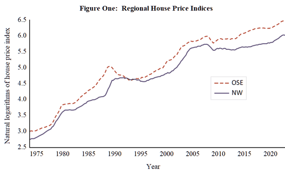
The results obtained from application of the DF-GLS test to OSE and NW are reported in Tables Four and Five below. From inspection of these results, it can be seen that the unit root hypothesis is not rejected for either series at conventionally considered levels of significance. Although not reported here, application of the DF-GLS test to the first differences of these series using the intercept model resulted in rejection of the unit root hypothesis beyond the 1% level of significance. The checking of this inference can form a further empirical exercise to employ in the classroom. Therefore, on the basis of the results obtained, it is concluded that OSE and NW are unit root processes.
Table Four: Applying the DF-GLS test statistic to OSE
| Calculated DF-GLS test statistic | Critical Values | ||
| 1% | 5% | 10% | |
| −1.609177 | −3.4720 | −2.9400 | −2.6500 |
Table Five: Applying the DF-GLS test statistic to NW
| Calculated DF-GLS test statistic | Critical Values | ||
| 1% | 5% | 10% | |
| −1.117594 | −3.4696 | −2.9380 | −2.6480 |
With OSE and NW determined to be unit root processes at typically employed levels of significance, the analysis undertaken within the classroom could proceed to support understanding of p-values by employing the code in the previous section. For example, the results for NW can be reconsidered. Setting the sample size to 192 observations to match that employed in the analysis of NW, the code can be utilised to derive the finite-sample distribution of the DF-GLS statistic and via consultation of the ordered simulated test statistics in the vector ‘stats’ the p-value associated with the calculated test statistic value of −1.117594 can be derived. The p-value resulting from this is 0.835 or 83.5%, thus illustrating how far we are from rejecting the unit root null hypothesis at conventionally considered levels of significance.
With OSE and NW concluded to be unit root processes, the possibility that they share a long-run relationship can be explored by examining the integrated nature of the ratio of these series. This ratio is presented in Figure Two and given its non-trending nature, the DF-GLS test is applied to this series using the intercept model specification.
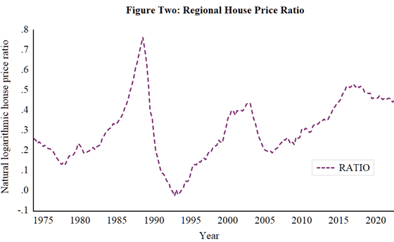
The results from application of the DF-GLS test to RATIO, again using the MAIC for lag optimisation, are reported in Table Six. he results obtained show that rejection of the unit root null hypothesis occurs beyond 1% level of significance. Consequently, evidence in support of the REH is apparent.
Table Six: DF-GLS test statistic and critical values
| Calculated DF-GLS test statistic | Critical Values | ||
| 1% | 5% | 10% | |
| −2.588555 | −2.5771 | −1.9425 | −1.6156 |
Linking to PedR
While active learning continues in this analysis, we have crucially added a research-driven dimension. Understanding of the DF-GLS test has to be transferred to its empirical application. Cognitive processing, in moving from underlying knowledge to its application in a particular context, is now fully observed. Students can be further challenged by asking how these results relate to pertinent published research, such as Meen (1999) and Cook (2005). Depending on the learning aims of the module, the analysis can then be extended to consider research on other economies and/or the use of alternative empirical methodologies. Investment in transferable skills are apparent in how data-related analysis relates to the creation and inspection of graphs, manipulation of series and undertaking of statistical analysis.
But, as before, the instructor should go beyond dictates over employability-related skills. In particular, the instructor has control over the extent of ‘discovery’ that is incorporated in the learning experience. They might choose extensive guidance and provide a ‘walk-through’. Alternatively, they might select an extreme form of a discovery-based approach. Here, students, directed to the Nationwide house price site and given the Meen (1999) quote, might be simply tasked to undertake ‘relevant analysis’. Clearly, options between these two extreme ‘guidance’ and ‘pure discovery’ forms can be employed.
5. Conclusion
A danger for adopting active learning methods in econometrics is to blind the participant with layers of the insipid. With the sector often adopting a ‘2+1’ lecture and computer lab format, a mechanistic approach can emerge. To avoid these deficiencies, the instructor should begin with a simple question: ‘how have I reflected on pedagogy to deliver my approach?’. That approach should be driven by a myriad of concerns: greater engagement; effective active learning; the development of transferable or employability-related skills; the building of self-efficacy and reduction of anxiety; and student research participation, rather than appearing as passive observers. The prominence of ‘action’ requires shedding of ‘Death by Powerpoint’ lectures. Consequently, we argue that, if possible, all sessions should be conducted within the computer lab. As a result, repeated activities and exercises can be undertaken that require the cognitive processing underlying meaningful learning.
Econometrics is about application. The task is to continually reflect upon ‘doing’.
References
Ashworth, J. and Parker, S. 1997. "Modelling regional house prices in the UK." Scottish Journal of Political Economy 44, 225-246. https://doi.org/10.1111/1467-9485.00055
Bandura, A. 1977. "Self-efficacy: toward a unifying theory of behavioral change." Psychological Review 84, 191-215. https://doi.org/10.1037/0033-295X.84.2.191
Cook, S. 2005. "Regional house price behaviour in the UK: Application of a joint testing procedure." Physica A 345, 611-621. https://doi.org/10.1016/j.physa.2004.07.031
Cook, S. and Watson, D. 2016. "A new perspective on the ripple effect in the UK housing market: Comovement, cyclical subsamples and alternative indices." Urban Studies 53, 3048-3062. https://doi.org/10.1177/0042098015610482
Cook, S. and Watson, D. 2023a. The use of online materials to support the development of quantitative skills, forthcoming in The Handbook of Teaching and Learning Social Research Methods, Nind, M. (ed.), Cheltenham: Edward Elgar.
Cook, S. and Watson, D. 2023b. "Crosswords and the ‘Active Learning’ Quest." Economics Network Ideas Bank. https://doi.org/10.53593/n3579a
Cook, S., Watson, D. and Vougas, D. 2019. "Solving the quantitative skills gap: a flexible learning call to arms!" Higher Education Pedagogies 4, 17-3 https://doi.org/10.1080/23752696.2018.1564880
Dickey, D. and Fuller, W. 1979. "Distribution of the estimators for autoregressive time series with a unit root." Journal of the American Statistical Association 74, 427-431. https://doi.org/10.1080/01621459.1979.10482531
Dowker, A., Sarkar A. and Looi, C. 2016. "Mathematics anxiety: what have we learned in 60 years?" Frontiers in Psychology 7, 508 https://doi.org/10.3389/fpsyg.2016.00508
Dreger R. and Aiken L. 1957. "The identification of number anxiety in a college population." Journal of Educational Psychology 48, 344-351. https://doi.org/10.1037/h0045894
Elliott, G., Rothenberg, T. and Stock, J. 1996. "Efficient tests for an autoregressive unit root." Econometrica 64, 813-836. https://doi.org/10.2307/2171846
Hudson, C., Hudson, J. and Morley, B. 2018. "Differing house price linkages across UK regions: A multi-dimensional recursive ripple model." Urban Studies 55, 1636-1654. https://doi.org/10.1177/0042098017700804
Jenkins, C. and Lane, S. Employability skills in UK Economics Degrees: A report for the Economics Network. https://doi.org/10.53593/n3245a
Lefrancois, G. 1997. Psychology for teachers (9th ed). Belmont: Wadsworth.
MacDonald, R. and Taylor, M. 1993. "Regional house prices in Britain: Long-run relationships and Short-Run Dynamics." Scottish Journal of Political Economy 40, 43-55. https://doi.org/10.1111/j.1467-9485.1993.tb00636.x
Mayer, R. 2004. "Should there be a three-strikes rule against pure discovery learning?" American Psychologist 59, 14-19. https://doi.org/10.1037/0003-066X.59.1.14
Mayer, R. 2021. Multimedia Learning (3rd edition). Cambridge: Cambridge University Press.
Meen, G. 1999. "Regional house prices and the ripple effect: A new interpretation." Housing Studies 14, 733-753. https://doi.org/10.1080/02673039982524
Müller, U. and Elliott, G. 2003. "Tests for unit roots and the initial condition." Econometrica 71, 1269-1286. https://doi.org/10.1111/1468-0262.00447
Ng, S. and Perron, P. 2001. "Lag length selection and the construction of unit root tests with good size and power." Econometrica 69, 1519-1554. https://doi.org/10.1111/1468-0262.00256
Peterson, W., Holly, S., Gaudoin, P., 2002. "Further Work on an Economic Model of the Demand for Social Housing." Report to the Department for the Environment, Transport and the Regions, London.
Phillips, D. 1998. "How, why, what, when, and where: Perspectives on constructivism in psychology and education." Issues in Education 3, 151-194.
Zahaciva, A., Lynch, S. and Espenshade, T. 2005. "Self-efficacy, stress, and academic success in college." Research in Higher Education 46, 677-706. https://doi.org/10.1007/s11162-004-4139-z
↑ Top