Alternative exercises to develop understanding of diagnostic testing
1. Introduction
Cook et al. (2025) advocate using simplified examples with bespoke, artificially generated data to support the teaching of simple linear regression. Set within a replication framework, this approach helps learners focus on specific topics by minimising complexities and removing extraneous factors. This paper draws motivation from Cook et al.’s (2025) discussion of the Expertise Reversal Effect (ERE, see Kalyuga et al. 2003) to develop exercises that challenge and enhance understanding of diagnostic testing in linear regression models, specifically addressing the issues of serial correlation and heteroskedasticity. Building on the ERE’s proposal that exercises should align with learners’ knowledge and experience, this paper introduces an alternative perspective on diagnostic testing that goes beyond typical approaches.
The case study builds on Cook et al. (2025) in two principal ways. First, we adopt their suggestion to use bespoke artificial data, carefully designed to highlight key features relevant to the concepts being explored. This strategy ensures that learners can focus on critical issues without unnecessary distractions. Second, inspired by their discussion of the ERE, the exercises are designed to suit different stages of the learning process, offering new perspectives to deepen understanding after initial exposure. The exercises adopt a distinct format that encourages exploration of specific issues in diagnostic testing. To illustrate this approach, we present three examples to support the learning of serial correlation and heteroskedasticity. Each exercise is accompanied by a discussion of its motivation and a detailed solution.
2. Example 1
Motivation
This example is designed to deepen understanding of the difference between positive and negative serial correlation, the structure of the Durbin-Watson (DW) statistic, and the relationship between the nature of serial correlation and the value of the DW statistic. Rather than following the familiar approach of testing for serial correlation by comparing the DW statistic to critical bounds at a given level of significance, the question challenges learners to identify, interpret, and synthesise information presented in graphs and specific elements of empirical output.
Question
An investigator estimated two models, referred to as Model A and Model B, specified as follows:
![]()
![]()
The estimation of these models produced the results presented in Tables One and Two. An examination of the residuals from the two models yielded the results shown in Figure One. Panel A of the figure displays a plot of the residual series from one of the regressions against its one period lag, while Panel B shows a corresponding plot for the other residual series.
Table One Dependent Variable: Y1 Method: Least Squares Sample: 1950 2023 Included observations: 74 | |||||||
| Variable | Coefficient | Std. Error | t-Statistic | Prob. | |||
| C | 1.927838 | 0.189425 | 10.17733 | 0.0000 | |||
| X1 | 1.085068 | 0.176790 | 6.137601 | 0.0000 | |||
| R-squared | 0.343486 | Mean dependent var | 1.872255 | ||||
| Adjusted R-squared | 0.334368 | S.D. dependent var | 1.994980 | ||||
| S.E. of regression | 1.627630 | Akaike info criterion | 3.838783 | ||||
| Sum squared resid | 190.7410 | Schwarz criterion | 3.901055 | ||||
| Log likelihood | −140.0350 | Hannan-Quinn criter. | 3.863624 | ||||
| F-statistic | 37.67015 | Durbin-Watson stat | 3.471770 | ||||
| Prob(F-statistic) | 0.000000 | ||||||
Table Two Dependent Variable: Y2 Method: Least Squares Sample: 1950 2023 Included observations: 74 | |||||||
| Variable | Coefficient | Std. Error | t-Statistic | Prob. | |||
| C | 1.148509 | 0.267430 | 4.294613 | 0.0001 | |||
| X2 | 1.652931 | 0.264133 | 6.257955 | 0.0000 | |||
| R-squared | 0.352297 | Mean dependent var | 1.334480 | ||||
| Adjusted R-squared | 0.343301 | S.D. dependent var | 2.821271 | ||||
| S.E. of regression | 2.286273 | Akaike info criterion | 4.518378 | ||||
| Sum squared resid | 376.3473 | Schwarz criterion | 4.580650 | ||||
| Log likelihood | −165.1800 | Hannan-Quinn criter. | 4.543219 | ||||
| F-statistic | 39.16200 | Durbin-Watson stat | 0.260522 | ||||
| Prob(F-statistic) | 0.000000 | ||||||
Figure One
| Panel A | Panel B |
|---|---|
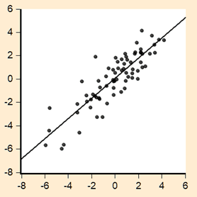 | 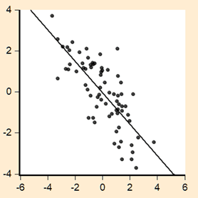 |
Using the above information, determine which residual series is depicted in Panel A and which is shown in Panel B.
Answer
This question requires synthesising knowledge from various aspects of the information provided above. One suggested approach is as follows: an understanding of the information in Figure One should lead to recognising that Panel A depicts positive residual serial correlation, while Panel B shows negative serial correlation. The relationship ![]() where
where ![]() represents the estimated first-order autoregressive parameter can be drawn upon to identify that the DW statistic reported in Table One indicates negative serial correlation, while the value in Table Two corresponds to positive serial correlation. Therefore, it can be concluded that Panel A represents residuals from Model B, and Panel B represents residuals from Model A.
represents the estimated first-order autoregressive parameter can be drawn upon to identify that the DW statistic reported in Table One indicates negative serial correlation, while the value in Table Two corresponds to positive serial correlation. Therefore, it can be concluded that Panel A represents residuals from Model B, and Panel B represents residuals from Model A.
As with other examples presented here, this discussion can be extended to address issues beyond the specific requirements of the task. For this example, a natural extension would involve formal testing of serial correlation by comparing the reported DW statistics to the critical bounds values. At the 5% level of significance, the relevant critical values for the sample of 74 observations can be interpolated as dL = 1.595, dU = 1.650, 4 − dU = 2.350 and 4 − dL = 2.405. These critical values lead to rejecting the null hypothesis of no serial correlation for both Models A and B, in favour of alternatives indicating negative and positive serial correlation, respectively. Furthermore, using the approximation for the DW statistic, additional exercises can be undertaken involving derivation of the approximated estimated values of ![]() as −0.736 for Model A and 0.870 for Model B.
as −0.736 for Model A and 0.870 for Model B.
3. Example 2
Motivation
This example presents results of applying a test for higher-order serial correlation. Rather than adopting a standard design that, for example, asks for inferences to be drawn from the provided information, the question focuses on the mechanical issues of test statistics and their application. This approach allows for the exploration of underlying intuition and the foundational principles behind the construction of these tests.
Question
Following the estimation of the simple linear regression model ![]() , an investigator conducted the analysis reported in Table Three below, where ‘RESID’ denotes the residual series
, an investigator conducted the analysis reported in Table Three below, where ‘RESID’ denotes the residual series ![]() . State the missing values denoted as Q, R and S in the output below.
. State the missing values denoted as Q, R and S in the output below.
Table Three Breusch-Godfrey Serial Correlation LM Test: Null hypothesis: No serial correlation at up to 4 lags | |||
| F-statistic | 7.908937 | Prob. F(Q,R) | 0.0000 |
| Obs*R-squared | S | Prob. Chi-Square(4) | 0.0001 |
Test Equation: Dependent Variable: RESID Method: Least Squares Sample: 1954 2023 Included observations: 70 Presample missing value lagged residuals set to zero. | |||||||||||
| Variable | Coefficient | Std. Error | t-Statistic | Prob. | |||||||
| C | −0.033487 | 0.054221 | −0.617598 | 0.5390 | |||||||
| X | −0.012620 | 0.052384 | −0.240912 | 0.8104 | |||||||
| RESID(-1) | 0.337973 | 0.121237 | 2.787708 | 0.0070 | |||||||
| RESID(-2) | 0.037143 | 0.135604 | 0.273909 | 0.7850 | |||||||
| RESID(-3) | 0.190195 | 0.136422 | 1.394168 | 0.1681 | |||||||
| RESID(-4) | 0.297190 | 0.135936 | 2.186254 | 0.0325 | |||||||
| R-squared | 0.330794 | Mean dependent var | 1.05E-16 | ||||||||
| Adjusted R-squared | 0.278512 | S.D. dependent var | 0.524406 | ||||||||
| S.E. of regression | 0.445433 | Akaike info criterion | 1.302275 | ||||||||
| Sum squared resid | 12.69825 | Schwarz criterion | 1.495003 | ||||||||
| Log likelihood | −39.57961 | Hannan-Quinn criter. | 1.378829 | ||||||||
| F-statistic | 6.327149 | Durbin-Watson stat | 2.106948 | ||||||||
| Prob(F-statistic) | 0.000079 | ||||||||||
Answer
This question can be approached as follows. The results in the above table pertain to testing for fourth order serial correlation, which is evident from the regression of RESID upon RESID(-1) through RESID(-4). The significance of the lagged residuals is the primary focus here, and the F-form of the Breusch-Godfrey test has 4 as its first degree of freedom given the four lagged residual terms. The second degree of freedom is 64, given the 6 regressors in the reported auxiliary regression and a sample size of 70 observations. These are the values of Q and R respectively. The missing value for S is given as 23.16 (to two decimal places), obtained using the chi-squared form of the statistic, defined as T × R2 from the auxiliary regression. By considering the degrees of freedom of the F-statistic, attention is drawn to the terms of interest in the auxiliary regression, highlighting the intuition behind the test —whether the lagged residual terms are significant— and the general construction of the test statistic. When determining the missing value S, the chi-squared form of the test is considered both in terms of its construction and its reliance on the auxiliary regression.
This example also lends itself to a broader exercise in hypothesis testing. While the reported p-values can be straightforwardly used to draw inferences, the structure of the question encourages exploring two perspectives on hypothesis testing using the traditional critical value vs. calculated statistic approach. The F-form of the test provides the calculated test statistic but requires finding missing values to derive a critical values. In contrast, the chi-squared form offers sufficient information to derive critical values directly, while the test statistic itself is absent.
4. Example 3
Motivation
Diagnostic testing and the residual sum of squares (RSS) are familiar components of regression analysis. Questions involving these elements often follow standard formats such as ‘exercise in substitution’ or ‘direct interpretation’: for example, the RSS might be employed in a formula to calculate a statistic, or the results of diagnostic testing might be presented to evaluate a model’s properties. This example, however, adopts a different approach: information from a secondary analysis is provided, and the task is to identify an undisclosed original model upon which this analysis is based and determine its RSS, which has not been explicitly provided. Additionally, the mechanics of hypothesis testing using White’s test of heteroskedasticity are reinforced by requiring the calculation of unreported test statistics. In both cases, solving the question involves extracting the appropriate information from the output provided and applying it correctly. The aim of this example is to deepen understanding of the mechanics of the diagnostic test in question and its two-stage nature, which involves an originally estimated model followed by a subsequent secondary regression.
Question
Suppose that, after estimating a multiple linear regression model for the variable Y, an investigator decided to examine its properties by applying White’s test for heteroskedasticity using cross-product terms. The results of this diagnostic testing are shown in Table Four below. Based on this information, state the residual sum of squares (RSS) of the originally estimated model and the calculated values of White’s test in both its F- and chi-squared forms (i.e. the missing elements denoted as A and B, respectively, in Table Four below).
Table Four Heteroskedasticity Test: White Null hypothesis: Homoskedasticity | |||
| F-statistic | A | Prob. F(5,94) | 0.0000 |
| Obs*R-squared | B | Prob. Chi-Square(5) | 0.0000 |
| Scaled explained SS | 147.3407 | Prob. Chi-Square(5) | 0.0000 |
Test Equation: Dependent Variable: RESID^2 Method: Least Squares Sample: 1 100 Included observations: 100 | |||||||||
| Variable | Coefficient | Std. Error | t-Statistic | Prob. | |||||
| C | 27.76544 | 18.15458 | 1.529390 | 0.1295 | |||||
| X^2 | 42.40738 | 17.36224 | 2.442507 | 0.0165 | |||||
| X*Z | 39.55390 | 18.00313 | 2.197057 | 0.0305 | |||||
| X | −87.37481 | 34.12831 | −2.560186 | 0.0121 | |||||
| Z^2 | 38.12609 | 12.82538 | 2.972706 | 0.0037 | |||||
| Z | −42.45490 | 31.80174 | −1.334987 | 0.1851 | |||||
| R-squared | 0.479211 | Mean dependent var | 30.04266 | ||||||
| Adjusted R-squared | 0.451510 | S.D. dependent var | 77.19017 | ||||||
| S.E. of regression | 57.16715 | Akaike info criterion | 10.98796 | ||||||
| Sum squared resid | 307199.8 | Schwarz criterion | 11.14427 | ||||||
| Log likelihood | −543.3980 | Hannan-Quinn criter. | 11.05122 | ||||||
| F-statistic | 17.29908 | Durbin-Watson stat | 2.213675 | ||||||
| Prob(F-statistic) | 0.000000 | ||||||||
Answer
An approach to answering this question is as follows: White’s test evaluates potential heteroskedasticity as a function of the regressors in the model under consideration. From the application of the test in its cross-product form, as shown in the table above, we can deduce that the original model contained two regressors (X, Z). Although the RSS for the original model is not explicitly stated, White’s test uses the squared residuals from this model as the dependent variable. The mean of this dependent variable is provided above (30.04266) along with the sample size (100). Therefore, with the mean of the squared residuals from the originally estimated model being 30.04266 over a sample of 100, the RSS of the originally estimated model is calculated as 3004.266 (to three decimal places).
Considering the missing values for the two statistics, the missing value for the F-form of the test statistic (denoted as A) pertains to the significance of the regressors terms, excluding the intercept term. This can therefore be calculated as:

The missing value for the chi-squared, denoted as B, is simply calculated as T × R2 = 47.9211.
5. Concluding remarks
This paper has proposed a series of exercises to support learning about diagnostic testing in linear regression. The approach taken draws upon Cook et al. (2025) and the concept of the Expertise Reversal Effect, with the exercises structured around the use of bespoke, artificially generated data. The proposed structure aims to complement more conventional exercises, such as the routine analysis of output to draw inferences. By requiring learners to engage with material from an alternative perspective, these exercises may be better suitable for later stages of the learning process, following the use of more traditional introductory activities.
These exercises not only enhance understanding of key diagnostic concepts such as serial correlation and heteroskedasticity but also encourage deeper engagement with the mechanics of hypothesis testing and model evaluation. By fostering analytical thinking and adaptability, the approach equips learners with a stronger foundation for tackling more complex real-world regression problems. Future research could explore the effectiveness of these exercises in diverse learning environments, further refining the tools available for teaching regression diagnostics.
References
Cook, S., Dawson, P. and Watson, D. 2025. Bridging the quantitative skills gap: Teaching simple linear regression via simplicity and structured replication. The Handbook for Economics Lecturers. Bristol: The Economics Network. https://doi.org/10.53593/n4229a
Kalyuga, S., Ayres, P., Chandler, P. and Sweller, J. 2003. Expertise reversal effect. Educational Psychologist 38, 23-31. https://doi.org/10.1207/S15326985EP3801_4
↑ Top