Volume 14, Issue 2, 2000
Teaching the Ramsey Growth Model using Linked Mathcad Worksheets
- Paul Turner
- Department of Economics, University of Sheffield
Introduction
Ramsey's (1928) model of optimal economic growth has, over the last 10-15 years, become the central organising framework of mainstream macroeconomic research. However, large numbers of postgraduate students and even more undergraduates remain largely unaware of its influence or even its existence. The reason is simple-the Ramsey model requires a level of mathematical technique which is well beyond that taught in most mainstream undergraduate economics degrees.
Such a disparity between the models used for research and those taught to students should be a matter for concern. Even if we cannot convey the full mathematical complexity of a model to students, surely we should at least try to convey to them the flavour of its results and its implications for the subject as a whole. In this paper, I will set up a possible route by which this can be achieved using linked Mathcad worksheets. The aim is to enable the problem to be studied at two levels-one worksheet solves the full mathematical problem, thus giving a level of treatment appropriate for postgraduate students, while the second hides the mathematical detail in favour of examining of the responses of the main variables of the system to changes in the parameters of the system. This second level could be used to convey the main points of the model to undergraduate students without alienating them by the use of complicated mathematics.
The problem to be solved can be stated as follows: a central planner wishes to choose time paths for consumption, investment and the capital stock which maximise the utility of a representative agent in the economy. The planner's objective function is therefore given by equation (1) with the capital accumulation equation (2) acting as a constraint.
![]() (1)
(1)
![]() (2)
(2)
where u(ct)is
the instantaneous utility function, which is assumed to be
non-negative, concave and increasing in consumption per capita ct,
q
is the discount rate and f(kt) is
the per capita production function, which is strictly concave in
capital per head kt and has the properties f(0) = 0, f´(0) = ![]() , f´(
, f´(![]() ) = 0.
The labour force is assumed to grow at constant proportional rate n.
As well as the constraint (2), the planner must also take into account
an initial condition that the capital stock is fixed at date zero and
a transversality constraint
) = 0.
The labour force is assumed to grow at constant proportional rate n.
As well as the constraint (2), the planner must also take into account
an initial condition that the capital stock is fixed at date zero and
a transversality constraint ![]() )
)
Mathematical solution
Suppose the utility function takes the constant relative risk
aversion form ![]() and the production function is Cobb-Douglas
and the production function is Cobb-Douglas
![]() (3)
(3)
where
![]() le-(1-g)/g,
le-(1-g)/g,![]() where
f1 is
the negative root of the characteristic polynomial of equation (3).
where
f1 is
the negative root of the characteristic polynomial of equation (3).
Solving the dynamic problem with Mathcad
To solve equation (3), we first use Mathcad to set values for the parameters of the system and then solve for values of k and l which are consistent with a stationary equilibrium as shown in Table 1. Note that this also enables us to solve for the steady-state values of income per capita ye and consumption per capita ce.
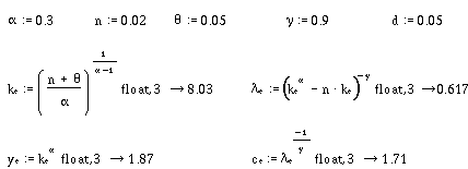
Table 1 Steady-state solution
Next we solve the differential equation (3) using the statements set out in Table 2. We first calculate values for a1,a2,b1,b2 then set x to be a vector of initial values for k and its derivative with respect to time. We then solve the equation by setting out the second-order differential equation (3) in the D vector and then using the rkfixed command which solves the resulting system using the Runge-Kutta method.
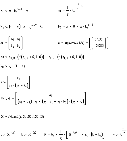
Table 2 Solution of the differential equation
Illustrating the solution with Mathcad
While the solution set out in the previous section might be appropriate for a mathematical economics or postgraduate macroeconomics course, it is unlikely that it would be appreciated by an undergraduate economics audience. Such students need to become familiar with the qualitative nature of the solution to the Ramsey model without getting trapped in the complexities of the mathematical solution. We can achieve this by making use of the Mathcad facility for linking worksheets. What we do is to set out the solution method outlined above in one worksheet and then link to it within another worksheet in order to illustrate the effects of changing the parameter values on the solution path. Particular important results that students should be aware of are as follows:
- Starting from a steady-state equilibrium, an increase in the growth rate of the labour force will initially increase consumption per capita, but in the long term both capital and consumption per head will fall.
- Starting from a steady-state equilibrium, an increase in the discount rate will produce a short-run increase in consumption, but in the long run the capital stock per head will fall and so will consumption per head.
- Starting from a steady-state equilibrium, an increase in the exponent on capital in the production function will have no short-run impact on capital and consumption per head, but both will increase in the long run.
- An increase in the coefficient of risk aversion g has no long-run effect on capital or consumption per head and will affect their dynamic paths only if the economy is out of steady-state equilibrium at the start of the simulation period.
Table 3 illustrates the process by which we can compute the effects of a change in one of the parameters on the model's dynamic path. In the first part, we set the values of the parameters, compute the equilibrium and set the initial value of the capital stock. We then call on the solution worksheet (Table 2) to compute the time path of the variables of interest and store each of these with the subscript b for base run. The coefficient d sets the initial proportional deviation of the capital stock from equilibrium, and the economy is assumed to begin in steady-state with d = 0. We then change one or more of the parameters, recalculate the equilibrium and call on the solution worksheet again to recalculate the dynamic path of the economy.
The graphs at the bottom of Table 3 illustrate the effects on the time paths of capital and consumption of a rise in the growth rate of labour from 2% to 3%. This produces a gradual fall in the capital stock until it reaches a new steady - state about 17.3% below its initial value. Consumption initially rises by about 5.5%, reflecting the greater weight put on current consumption. In the long run, it falls by about 5% as the capital stock and output both fall. The initial increase in consumption may seem surprising given the diminishing returns to labour embodied in the production function. What is happening is that, when labour growth increases, the central planner realises that the long-run level of capital per head will fall and allows households to start consuming some of the existing capital stock. This is enough to generate a short-run increase in consumption per head despite the increased growth rate of the labour force. In the long term, the fall in the capital stock produces the fall in output and consumption per head that we would intuitively predict for this model.
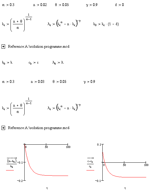
Table 3 Solution worksheet illustrating effect of an increase in the
growth rate of labour
In Table 4 we illustrate the effects of an increase in the discount rate and an increase in the exponent on capital in the production function. An increase in the discount rate produces effects similar to an increase in the growth rate of the labour force. Capital per head falls in the long run, while consumption initially increases and then falls. An increase in the exponent on capital is equivalent to a long-run increase in the marginal productivity of capital. Its effects are to increase the equilibrium level of capital and consumption per head, but there is no short-run response in either variable.
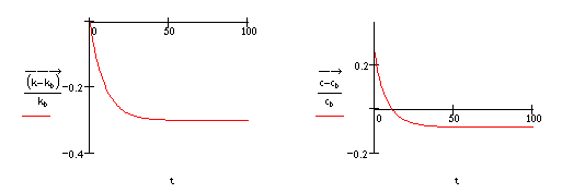
Increase in the discount rate from 5% to 7%
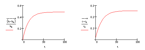
Increase in the exponent on capital from 0.3 to 0.35
Table 4 Dynamic effects of changes in model parameters
Finally, we consider the effects of an increase in the coefficient of relative risk aversion g. This amounts to an increase in the curvature of the instantaneous utility function. It is straightforward to show that this has no effect on the steady-state levels of either capital or consumption per head. Therefore, if the economy is initially in steady-state equilibrium, it simply remains there. However, if the economy is not initially in steady - state, an increase in g will affect its dynamic path to equilibrium. In Table 5, we show the effects of an increase in g from 0.9 to 1.0, on the time paths of capital and consumption when capital is initially 5% below equilibrium. In the short run the level of capital falls below its base path before rising back towards it. Corresponding to this, there is a short-run increase in consumption before it too falls below its steady-state value and then converges to equilibrium.

Table 5
Effects of an increase in the coefficient of relative risk aversion
Summary
In this paper, I have shown how Mathcad can be used to solve for local dynamic behaviour of capital and consumption in the Ramsey growth model. The model is solved explicitly using the linearised second-order differential equation for capital, the initial condition for the capital stock and the transversality condition. I have also shown how the comparative dynamic properties of the model can be illustrated using Mathcad in order to aid the teaching of a complex model to an undergraduate macroeconomics principles class. Copies of the Mathcad worksheets used in this paper can be downloaded from my web page at the following URL: http://www.shef.ac.uk/~ptn/downloads/download.htm
References
Blanchard, Olivier J. and Stanley Fischer (1989) Lectures on Macroeconomics, Cambridge,MA: MIT Press.
Murphy, Barry (1996a) 'Mathcad Plus 5.0: a review', Economic Journal, vol. 106, no. 437, pp. 1115-22.
Murphy, Barry (1996b) 'Mathcad 6.0', CHEER, vol. 10, no. 2, pp. 20-3.
Ramsey, Frank P. (1928) 'A mathematical theory of saving', Economic Journal, vol. 38, no. 152, pp. 543-59.
Contact details:
Dr P. M. TurnerDepartment of Economics
University of Sheffield
9 Mappin Street
Sheffield S1 4DT
UK Tel: 0114 2223404
Email: p.turner@sheffield.ac.uk

