Volume 10 Issue 3, 1996
Economic Optimisation: An Excel Alternative to Estelles et al's GAMS Approach
- Ziggy MacDonald
- University of Leicester
Introduction
In a recent edition of CHEER Estelles et al (1996) presented a paper discussing an approach to teaching economic optimisation using the GAMS (General Algebraic Modelling System) software. GAMS is a powerful modelling language which can cope with very large programming problems of varying types (e.g. integer, non-linear, etc.). The fact that it is a high level language is perhaps the reason that drives me to question its suitability as a teaching tool. Although students should be encouraged to explore a variety of problem solving tools, thus widening their portfolio of skills, my suspicions are aroused when the tool requires the user to employ two applications in order to generate the output from one application. Such is the case with solvers such as GAMS where an input file containing the instructions for the solver has to be created in a third party text editor. Having run the input file through the solver an output file is generated which, of course, then has to be viewed in a text editor.The purpose of this response to Estelles et al is to show that not only is a common place Windows spreadsheet such as Excel far friendlier for students to use, it also allows greater flexibility and speed for post-optimality analysis. The strong appeal of Excel Solver lies in its ease of use and the enlightening nature of spreadsheet work, a point echoed by Hillier & Lieberman (1995), who in discussing the arrival of spreadsheets solvers such as excel, commented that "the convenient data entry and editing features of spreadsheets also are very helpful in constructing linear programming models" (p 131). In addition, many students on UK campuses have a sound grounding in the basic use of Excel as it is the industry standard spreadsheet and spreadsheet use has been widely encouraged in economics education for years (e.g. Judge 1990, Judge 1996). Thus, unlike with GAMS, the student does not have to become familiar with a new syntax or procedure for declaring variables and accessing routines. The recognition of the potential of Excel Solver is also starting to appear in textbooks, particularly Hanna (1996), where others have traditionally relied on LINDO as the standard instructional software (e.g. Wilkes 1989, Winston 1995, Ravindran et al 1987).
Using Excel Solver
Optimisation in Excel is achieved via the Solver Add-In (installed in Excel from the menu option Tools | Add_Ins and subsequently accessed from the menu option Tools | Solver). The basic process of setting up an optimisation problem is discussed in detail in MacDonald (1995) but essentially it requires the user to use cell formulae to relate the objective function and constraints to cells that are designated as 'changing cells' i.e. the decision variables. To illustrate this, consider the example used in Estelles et al, given in Problem 1. This is a simple 'diet problem' in which the cost of purchase (C) of two foods (x1, and x2) has to be minimised subject to the provision of the correct daily nutrient requirement (assumed to be only calcium, protein and vitamin A) acquired from their consumption.
Problem 1: A Simple LP
(Note 1)
| Min C = 0.6x1 + x2 | ||
| s.t. | 10x1 + 4x2 >= 20 | (calcium) |
| 5x1 + 5x2 >= 20 | (protein) |
|
| 2x1 + 6x2 >= 12 | (vitaminA) |
|
| x1,x2 >= 0 | |
|

Figure 1
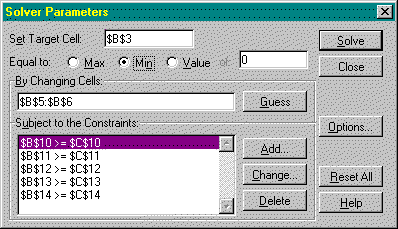
Having set-up the cell formulas in the spreadsheet, the user then has to reference the problem in the Solver dialogue box (shown in Figure 2) and simply click 'Solve'.

Figure 2
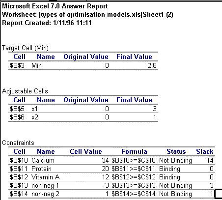
Unlike GAMS, where the problem solution is buried in a large output file, on clicking 'Solve' the answer is quickly revealed in the spreadsheet cells and an option to create an answer and sensitivity report is provided. The answer report for this simple problem is given in Figure 3.

Figure 3
The answer report reveals not only information about the optimal solution but also the status of the constraints. Should the user get an unexpected answer, the report is also useful for debugging as the constraint formulas are given (although it is just as simple to select the Solver and check them in there).
Post-Optimality Analysis
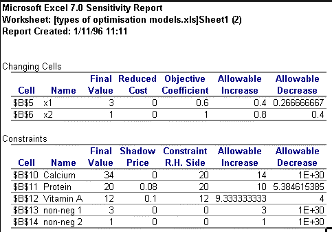
One of the real advantages of Excel is the ease with which post-optimality analysis can be executed. The relevance of the range of optimality for objective coefficients and the meaning of shadow prices rarely appears to filter through to students when first discussed in a lecture. Sitting in front of Excel, however, and the subject comes to life, and this is possibly the most significant distinguishing feature between Solver and GAMS. The problem with GAMS as a teaching aid is that in order to illustrate the effect of incremental changes in, say, objective coefficients, and in particular, to illustrate the 100% rule, the user has to go in and out of a text editor several times. In Excel the process is smooth and instantly revealing. Consider the example illustrated above. The answer and sensitivity reports are generated in the worksheets adjacent to the original problem. Provided the user has selected "Assume Linear Model" from the Option dialogue box, the sensitivity report provides information on allowable ranges for objective function coefficients and RHS values in addition to the usual reduced cost and shadow price information. The sensitivity report for the problem illustrated above is provided in Figure 4.

Figure 4
Consider changing the price of good 1 (x1) from 0.6 to 0.9. The sensitivity report reveals that this is within the range of optimality (i.e. below the maximum allowable increase) and so the optimal values of x1 and x2 should remain unchanged. To test this the student has only to change the one cell in the spreadsheet, click to solve again and the new value for cost and the unchanged decision variables appear instantly (x1 = 3, x2 = 1, C = 3.7). Given this simplicity it is yet more revealing when students put the 100% rule to test (i.e. that for a simultaneous change in objective coefficients, provided the sum of the changes as expressed as a percentage of the corresponding allowable increase/decrease does not exceed 100% the optimal values of x1 and x2 should not change (Note2)). What is more, exploring the meaning of the shadow prices given in the sensitivity report is equally as simple because the RHS values for each constraint are given in separate cells in the spreadsheet. A simple change to the RHS of the protein constraint (the only binding constraint in this problem), say to a requirement of 21 units per day, will reveal to the student, on re-solving, an increase in cost of 0.08, as predicted by the shadow price. As with the objective coefficients, the student could then proceed to test the allowable range for the RHS values by resolving and generating new sensitivity reports to observe the effect on the shadow price.
Types of Optimisation
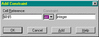
Not only is observing the effects of model re-specification a simple and straightforward process, it is equally as simple to modify the type of optimisation being considered. In most cases you do not have to specify the type of optimisation you wish Excel Solver to undertake. Referring back to the simple diet problem, it is perhaps realistic to assume that only integer values should be used for the daily consumption of the two foods (although, fortunately, the optimal solution is already integer). Assuming the integer requirement was necessary, as would be the case if the price of good one were £1 rather than 60p, all that is required is to add two further constraints in the Solver dialogue box, shown in Figure 5, which reference the changing cells (the decision variables) and force them to integer.

Figure 5
A particularly useful feature of Excel Solver is the option to have the solution paused at each iteration. This is achieved from the 'Options' button in the Solver dialogue box by checking the option 'Show Iterations'. If we make the change to the original diet problem so that the cost of good one is £1, then using this option the student can see that the LP solution takes 6 iterations. Forcing the changing cells to take integer values then requires 15 iterations to achieve the optimal integer solution. This option can really help students appreciate the computational requirements of integer problems. One example I use in my third year Optimisation in Business course is a simple 5 variable, 8 constraint profit max problem that requires only 6 iterations to solve as an LP. In the lecture I then force the integer requirement and the problem is dramatically transformed. Remembering to un-check the 'Show Iterations' option, the problem is solved after approximately 1000 iterations and around 340 branches, which the students can see occur at the bottom left of the Excel screen in the status bar. None of these facilities are available in real-time in GAMS. Although the GAMS output does provide detailed analysis of resource usage and iteration count, for example, this can only be accessed after the solution is completed and the student has read the output file into a text editor (and spend some time hunting the rather detailed output for this information and the solution, which is right at the end).
Finally, Excel Solver can easily accommodate non-linear or parameterised problems as it can linear and integer problems without any special modifications. Referring to the example in Estelles et al, given in Problem 2, the non-linear problem is entered into Solver in exactly the same way as a linear problem except that the option 'Assume Linear Model' must be un-checked in the Solver Options dialogue box.
- Problem 2
- min C = 4K + 5L
- s.t. 10 K0.5L0.5 >= 1000
- K,L >= 0
- s.t. 10 K0.5L0.5 >= 1000
Of course, further flexibility can be added to this type of problem by putting the parameters in separate cells which can be subsequently altered and the impact on the solution immediately observed.
Limitations
Although a fan of Excel Solver I'm not on commission and there some are problems with the routine, particularly with respect to reduced costs. From my experience of Solver it appears to be somewhat selective as to when it provides reduced cost values. The theory suggests that if a variable is not part of the basis in the solution then the reduced cost value should indicate the amount by which the coefficient has to improve (for a max problem) before that variable will enter the solution. If the reduced cost value for a non-basic variable is zero then this is an indication of the presence of alternate optima. The problem with Solver is that invariably the reduced costs for non-basic variables are zero when clearly there isn't an alternate optima and other packages provide values. This is clearly a problem as such information is the bread and butter of report writing for problems where not all variables form part of the solution.
Concluding Remarks
Excel Solver is very accessible to students and provides a rich environment in which to explore optimisation problems. Although GAMS can probably handle larger problems than Excel (as it is a modelling language and therefore specifically designed for the task), it is perhaps more cumbersome and certainly less self-contained. The flexibility of Excel Solver is one of its strongest attractions, particularly in respect of exploring post-optimality changes to the original problem. Although students have to be quite careful in defining the problem, in Excel debugging is very straightforward and can of course assist in the learning process. In conclusion, GAMS is clearly a sufficient medium in which to explore optimisation problems, however, problems with reduced cost aside, Excel Solver is better equipped to facilitate learning and will remain my preferred solver for teaching, and invariably, a firm favourite with students.
References
Chiang, A. C., 1984, "Fundamental Methods of Mathematical Economics", 3rd Edition, McGraw-HillEstelles, T. C., Arre, M. M. & Garrido, R. S., 1996, "Economic Optimisation with GAMS", Computers in Higher Education Economic Review, 10 (2) 2-7
Hanna, M., 1996, "Introduction to Management Science - Mastering Quantitative Analysis", South-Western
Hillier, F. & Lieberman, G., 1995, "Introduction to Operations Research", sixth edition, McGraw-Hill
Judge, G., 1990, "Quantitative Analysis for Economics and Business Using Lotus 1-2-3", Harvester-Wheatsheaf
Judge, G., 1996, "Student Created Spreadsheet Models for Teaching & Learning Economics: An initial Self-Evaluation of an Experimental Assignment", Computers in Higher Education Economic Review, 10 (2) 16-18
MacDonald, Z., 1995, "Teaching Linear Programming using Microsoft Excel Solver", Computers in Higher Education Economic Review, 9 (3) 7-10
Ravindran, A., Phillips, D. & Solberg, J., 1987, "Operations Research - Principles & Practice", 2nd Edition, Wiley
Wilkes, M., 1989, "Operational Research - Analysis & Applications", McGraw Hill
Winston, W. L., 1994, "Operations Research -Applications & Algorithms", 3rd Edition, Duxbury (Wadworth)
Ziggy MacDonald
Department of Economics
University of Leicester
University Road
Leicester. UK
LE1 7RH
E-mail abm1@le.ac.uk
Note 1: The model given in Estelles et al has a typo error: the RHS value of the 3rd constraint is shown as 20 whereas in Chiang's original problem (Chiang 1984 page 652) the RHS value is 12. Estelles et al have used the correct figure, however, in their computer solution and output.
Note 2: Although for small problems the sum can also safely far exceed 100% without affecting the optimal solution.
|
What's Related: · Other articles on the use of spreadsheets in teaching economics |

