Teaching the Economics of Non-renewable Resources to Undergraduates

William L. Holahan and Charles O. Kroncke
International Review of Economics Education, volume 3, issue 1 (2004), pp. 77-87
DOI: 10.1016/S1477-3880(15)30143-2 (Note that this link takes you to the Elsevier version of this paper)

Up: Home > Lecturer Resources > IREE > Volume 3 Issue 1

Abstract

Harold Hotelling’s path-breaking article in 1931 used higher mathematics to explain the economics of non-renewable resources. In that article, Hotelling asserted that conventional static models were inadequate to illustrate his ideas, and presumably he would have extended that opinion to the many technical papers that his work spawned.

The purpose of this paper is to show how to extend the conventional static model to enable instructors of economics to present to undergraduates at least some of the ideas of Hotelling and later research economists. By making such presentations, these introductory courses can make a great improvement in economic understanding at precisely the time in our history that energy policy in general, and oil dependence in particular, are front-page news.

JEL Classification: A22

Introduction

With the recent release of the NEPDG (National Energy Policy Development Group) Report, teachers of basic economics courses have an excellent opportunity to demonstrate how a proper understanding of economic principles is essential when making and analysing public policy. The NEPDG Report notes that domestic oil production declined for most years after 1970, offsetting increases in the production of coal, natural gas, nuclear and renewable energy. The report calls for significant departures from the market outcome, including several methods of subsidising the extraction of petroleum, such as modification of federal oil and gas leases, royalty reductions and more development offshore as well as in Alaska’s National Petroleum Reserve. It concludes that the United States needs such a change in order to reduce its dependence on foreign suppliers. Given the instability in the Middle East and the ability of OPEC to manipulate world prices, a policy that claims to reduce US vulnerability to these forces plays well with the American public.

The economics of oil must take into account that it is a depletable non-renewable resource.^{(note 1)} In his path-breaking 1931 article,^{(note 2)} Harold Hotelling recognised that the marginal cost of extraction of a non-renewable resource depends not only on the current rate of production but also on the amount of cumulative production (or equivalently, the stock remaining in the ground); however, he discounted the ability of economists to explain the economics of non-renewable resources without recourse to higher mathematics. He wrote:‘The static-equilibrium type of economic theory which is now so well developed is plainly inadequate for an industry in which the indefinite maintenance of a steady rate of production is a physical impossibility, and which is therefore bound to decline.’ An almost exclusive reliance on this static model in principles and intermediate microeconomics courses has laid a weak foundation for the presentation of the economics of depletable nonrenewable resources. Only a few students take the math required to read Hotelling’s work or the literature it has spawned.^{(note 3)}

This paper is an effort to show how a properly reworked version of the static model can indeed introduce students to the problems of depletable non-renewable resources and equips them, at an early stage in their study of economics, to understand the economics of oil. We suggest that the instructor introduce a new curve that rests both on the standard family of average and marginal cost curves, and on the ‘Hotelling Rule’ that describes how those costs are rising over time as the resource is extracted.^{(note 4)} By slightly extending the lectures on cost curves, the instructor’s presentation can demonstrate historic misunderstandings and help to identify the steps necessary for achieving a more market-oriented approach to energy policy.

Preliminaries

In order to explain the economics of oil and establish the way a market would allocate it over time, the material in this paper could be inserted in the course after the standard treatment of the ATC, AVC and MC curves, and the treatment of static competition. Many texts omit the equal-marginal-cost principle, which the instructor should also present first. We present a summary here.

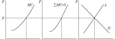
Figure 1 is the standard supply and demand picture illustrating the equal-marginal-cost principle. Each firm is a price taker, taking as given the price determined by market supply and demand. In a competitive market, each faces the same price and sets output so that marginal cost equals price. Since price is the same for all firms, they all have the same marginal costs. All of these principles are key to understanding the oil market.

Figure 1

(a)	(b)	(c)
qI Firm	∑qI Country	Q World

Total industry cost is minimised when marginal costs are equated.^{(note 5)} The proof is by contradiction: suppose one firm had a higher marginal cost than another. A rearrangement of a unit of output from the higher marginal cost firm to the lower marginal cost firm would result in no change in total output, but a reduction in total cost. To minimise total industry cost, all such opportunities to squeeze costs out must be seized until the marginal costs of all firms are the same. In a price system, this happens automatically when all firms follow the incentive to set marginal cost equal to the same price.

To model the world market as it would be if competitive, the student must understand the horizontal summation of marginal cost curves. Panel (a) of Figure 1 shows the marginal cost of the firm. Price is determined by supply and demand. Because each firm accepts price as given, the individual firm marginal cost curves can be summed to derive the country’s supply curve in panel (b). In panel (c), the supply curves in individual countries are summed to derive the supply curve for the world. In a price-taking world, output is produced at minimum cost.

Modifying the diagram to explain the oil market

To understand energy policy, this analysis needs to be modified to reflect the nonrenewable nature of oil resources. The market would induce firms to extract oil in a profit-maximising pattern: with the lowest marginal extraction cost first, and then to proceed to tap higher marginal cost reserves. (Marginal cost differs because oil reserves lie in geological structures that vary in location, weather, depth, pressure and other characteristics that impact on their extraction. Even within a single structure, different reserves may differ in marginal extraction costs.) Extraction continues until marginal cost rises to price. Reserves that could be extracted profitably at higher prices, but not current prices, remain in the ground, available in the future should prices rise or technological change reduce costs. That is, at all times, the decision to extract or store for the future depends on the comparison of marginal cost and price.

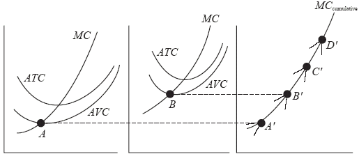
In Figure 2, we introduce a cumulative marginal cost curve that reflects the economics of oil extraction. The three panels of Figure 2 permit us to see how the marginal cost curves shift as oil is depleted from a geological structure. Panel (a) shows the family of cost curves in period 1, and panel (b) shows the family of cost curves in period 2. Note that these panels seem to depict a static family of curves at a point in time. However, taken in sequence, (a) first, then (b), they are actually depicting a dynamic process of extraction. Extraction causes the curves to rise due to depletion. Thus, in period 2, the curves have risen to positions higher than they were in period 1. We are deploying static figures to depict the choice of output at a moment in time, where the rate of output, in turn, determines the rate at which costs are rising – slow depletion causes the cost curves to rise slowly; rapid depletion causes the curves to rise rapidly.

Standard economic principles tell us that a firm will select its output to set marginal cost equal to price, or produce no output if price lies below minimum average variable costs. Thus, referring once again to Figure 2, the firm in period 1 will not operate if price lies below point A, and in period 2 will not operate if price lies below point B.When the firm has depleted a portion of its in-ground oil, it cannot get that oil a second time, and it cannot get its replacement at the same cost as it did in prior periods (cet. par., i.e. same technology).

Figure 2

(a)	(b)	(c)
Period 1 output of firm A	Period 2 output of firm A	Cumulative output

In panel (c), we have horizontally summed the marginal cost curves shown in panels (a) and (b) for periods 1 and 2. Point A' corresponds to point A in panel (a), therefore the height of A' is the minimum AVC in period 1. Point B' corresponds to point B in panel (b) and therefore the height of B' is the minimum AVC in period 2. Just as depletion raises the family of cost curves, it also makes portions of the cumulative marginal cost curve disappear. For example, as we make the transition from period 1 to period 2, the portion A'B' disappears. Although when we use paper we are forced to depict only discrete time periods, the process of oil depletion is steady rather than discrete.^{(note 6)} The cumulative marginal cost curves show this steady rise in marginal cost better than the time-specific families of cost curves. Students should learn that the steady elimination of the lower portion of the cumulative marginal cost curve (as if being chewed up by Pac Man) occurs because oil is being depleted.

Since the cumulative marginal cost is a function of all oil depleted from a structure up to a point in time, it is different in character from the conventional marginal cost curve, which is a function of the rate of output at a given point in time. The cumulative marginal cost curve is derived from conventional curves, but unlike the conventional curves, which a firm can ride up and down, the cumulative curve has a sense of direction: the firm can climb up the curve, but not back down as oil is depleted, precisely because oil is non-renewable. As a reminder of this fact, we place small upward-pointing arrows on the cumulative marginal cost curve. For example, once the oil whose marginal extraction cost is shown by point A' has been extracted, that portion of the cumulative marginal cost curve disappears. As depletion proceeds, the firm must pay higher and higher marginal costs to extract more oil. The upward-sloping cumulative marginal cost curve expresses the reality that the ‘easy oil is taken first’.^{(note 7)}

Cumulative marginal cost curves can be summed horizontally just as conventional marginal cost curves can. At any given price, the firms set output so that marginal cost equals price, so long as price is at least as great as minimum ATC. In Figure 3, we have a three-panel diagram that shows two representative firms in an industry and the industry summation marginal cost curve. In the figure, firm 1 will not produce output because the price is too low. Its oil will be preserved for the future when prices rise. Firm 2 will produce q_A at price P_A and the industry output is shown by the summation curve (of a large number of firms) with industry output of Q_A.Thus some firms are not producing, the rest are, and a rise in price will increase not only the total output of the industry but also the number of producing firms. Similarly, if price falls, perhaps due to discoveries of oil in Azerbaijan, then some firms will stop producing while others continue to produce, but at a lower rate of production.^{(note 8)}

Figure 3

(a)	(b)	(c)
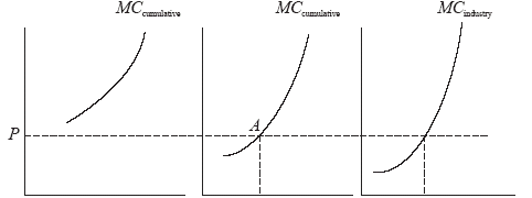
Firm 1	qa Firm 2	Qa Industry

If technological change occurs that reduces costs, the cumulative marginal costs fall and the industry marginal cost shifts to the right. More firms can produce at any given price. Similarly, if technological change occurs in the production of a substitute, such as natural gas liquefaction, the demand for oil will fall, reducing the price of oil and causing some firms to stop production and others to produce at a reduced rate.^{(note 9)}

US oil policy in light of oil’s non-renewable character

For years, US energy policy has subsidised the extraction of domestic oil, resulting in artificially low prices, more consumption and less public concern for the efficient use of oil and its substitutes. Worse, by skewing energy use to subsidised oil, the artificially low prices have deterred technological innovations and removed the motivation for research and development into energy alternatives, making the country even more dependent on oil. Higher-cost domestic oil that should have remained in the ground until world prices dictated otherwise was instead exhausted even though lower-cost oil could have been imported. The NEPDG recommendations continue this tradition. Using the cumulative cost curve in Figure 4, the instructor can demonstrate that such subsidies are an incentive to extract oil sooner than would be the case if competitive markets were allowed to prevail in the domestic oil industry.

In Figure 4, a cumulative marginal cost curve is shown in which the price is less than the marginal cost (A). From the previous analysis of Figure 2, we know that the firm will choose to shut down. Now suppose that the energy subsidies called for by NEPDG are available to the firm. Geometrically, this drives down the marginal cost that the firm perceives and so the operative curve is MC_cumulative minus subsidy.

Figure 4

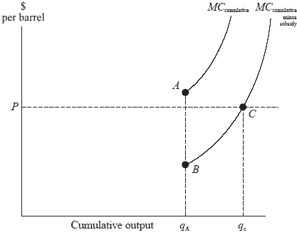
The minimum average variable cost at the cumulative depletion point q_A is now driven down to point B.Since point B lies well below price, the firm will now deplete oil that it would not have had the market price not been subsidised. The producer will extract oil at price P until MC_cumulative minus subsidy is driven up to point C. The subsidy policy will result in extra oil produced equal to q_C – q_A.That is the amount that would be left in the ground without the subsidy.

Without NEPDG incentives in effect, US marginal cost at A is above the world marginal cost. However, due to NEPDG subsidies, firms are encouraged to extract their more costly reserves. Consumers enjoy artificially reduced prices for petroleum-based energy, but as a nation, because of diminished domestic reserves, the United States actually becomes more dependent on foreign suppliers. Moreover, it is less able to react to the price spikes induced by supply disruptions. This analysis would imply that implementation of the NEPDG proposals will produce the opposite of their intended effect: rather than reducing the United States’ dependence on foreign oil, the policy would increase its dependence.

Because oil is a non-renewable resource, the United States actually becomes less dependent, not more dependent, when it imports. When price is less than domestic extraction costs, consuming another country’s oil is the correct decision. Dependency should not be defined as how much the United States is importing at a given moment, but rather how costly and how rapidly it could respond to price spikes caused by cartel price manipulations or war. The United States becomes less dependent when it lets the market dictate the pace at which the country uses domestic and foreign oil.^{(note 10)}

The impact of Russian oil on the world market

The best way to force a cartel to reduce its price is for additional oil to come on to the market. In recent years, Russia, long the owner of huge oil reserves but unable to bring much of it to market, has greatly improved its pipeline network and cooperates little with OPEC to keep prices high by restricting output. What does the cumulative marginal cost curve teach us about an efficient policy response to the emergence of Russia as a major oil exporter? Answer: as always, consult the marginal cost and the world price. If Russian oil is available for less than the unsubsidised marginal cost, it should be imported. Domestic reserves that cost more should remain in the ground.

‘Doesn’t this make the US more dependent on Russian oil?’ No more than we are dependent on their caviar! If they dramatically raised the price of caviar, we would find substitutes. Similarly, if we efficiently extract oil, leaving the efficient amount in the ground, the opportunity to substitute domestic oil exists if Russia decided to join OPEC. Again, the key consideration is that we are dependent on oil. Our dependence on foreign sources is home grown: by depleting our low-cost reserves, we have become more reliant on foreign sources than we would have been if we had let the market work. The proper response to lower-cost Russian oil – that is, import it as long as it is cheap – is completely at odds with the NEPDG policy recommendations. By expanding its sales on the world market, Russia has replaced some of the oil that OPEC withheld from the market and frustrated its efforts to boost prices. Now is the time to import this cheap foreign oil and to preserve the United States’ domestic reserves. We become less dependent when we let the market dictate the pace at which we use domestic and foreign oil.

What of ANWAR?

One of the NEPDG recommendations is to slate a tiny portion of the Alaskan Wildlife Refuge for exploration and oil production. Not surprisingly, this recommendation raises the ire of environmentalists who express concern for the pristine wilderness and for the animal life that may be disrupted. The cumulative marginal cost curve shows why, even if there were no environmental concerns, this oil should not be extracted: because such extraction can only occur if subsidised, it is too soon to extract it now. When extraction of such oil requires a subsidy, it cannot compete with cheap foreign oil. Simply put, it should remain in the ground. Environmental concerns are a separate issue.

Conclusion

The United States is dependent on oil, not foreign oil. Since oil is non-renewable, one must be careful in analysing that dependence. We should use foreign oil when it is cheap, and domestic oil during those periods when domestic oil is cheaper than the world price. To smooth the effects of sudden spikes in the world price of oil, the Strategic Petroleum Reserve should be full and ready to counter sudden production cuts. The rule for filling the SPR is the same as for any other use of oil: fill it with domestic oil when that is the cheaper source; fill it with foreign oil when that is cheaper.

Energy policy promises to be a hot topic for years to come. By presenting the issue in terms of cumulative marginal cost curves, we offer economics teachers another tool to help clarify their students’ economic understanding of this issue.

References

Deshmukh, S. and Pliska, S. (1980) ‘Optimal consumption and exploration of nonrenewable resources under uncertainty’, Econometrica, vol. 48, no. 1, pp. 177–200.

Devarajan, S. and Fisher, A. (1981) ‘Hotelling’s ‘Economics of exhaustible resources’: fifty years later’, Journal of Economic Literature, vol. 19, no. 1, pp. 65–73.

Gilbert, R. (1979) ‘Optimal depletion of an uncertain stock’, Review of Economic Studies, vol. 46, no. 1, pp. 47–57.

Hotelling, H. (1931) ‘The economics of exhaustible resources’, Journal of Political Economy, vol. 39, no. 2, pp. 137–75.

Mann, C. (2002) ‘Getting over OIL’, Technology Review, January/February, pp. 32–8.

National Energy Policy Development Group (2001) National Energy Policy: Reliable, Affordable, and Environmentally Sound Energy for America’s Future, Washington, DC: NEPDG.

Pesaran, M. (1990) ‘An econometric analysis of exploration and extraction of oil in the UK continental shelf’, Economic Journal, vol. 100, no. 401, pp. 367–90.

Pindyck, R. (1980) ‘Uncertainty and exhaustible resource markets’, Journal of Political Economy, vol. 88, no. 6, pp. 1203–25.

Pindyck, R. (1984) ‘Uncertainty in the theory of renewable resource markets’, Review of Economic Studies, vol. 51, no. 2, pp. 289–303.

Stiglitz, J. (1976) ‘Monopoly and the rate of extraction of exhaustible resources’, American Economic Review, vol. 66, no. 4, pp. 655–61.

Notes

[1] The distinction between ‘non-renewable’ and ‘exhaustible’ resources should be made at the outset. Exhaustible resources are those that can be all used up, but need not be. For example, steer and bison are exhaustible in the sense that, if they are all killed, no replacement is possible. If properly managed, however, these herds can grow: steer through market incentives and private property rights, and bison through government intervention, unless a market comes into existence sufficient to create similar incentives.‘Non-renewable’ adds an extra meaning to ‘exhaustible’: a unit of a non-renewable resource cannot be replaced and at any positive rate of use this resource will eventually be gone.

[2] Hotelling employed calculus of variations, not commonly understood by economists in 1931, but now common in graduate curricula. However, so seldom does an undergraduate understand such methods when taking principles or intermediate microeconomics that the course cannot utilise that mathematical analysis. Hence the topic is not presented at all in the majority of texts.

[3] Many papers have been written in the last two decades of an even more difficult nature. The simple technique provided here can only enable the instructor to whet students’ appetite for the intriguing economics of non-renewable resources. A fine review article by Devarajan and Fisher (1981) appeared 50 years after Hotelling’s article. The review manages to make his work a bit more understandable, but still does not help much to explain the analysis to students who will take only principles courses or perhaps intermediate micro. Additional articles on this topic include Deshmukh and Pliska (1980), Gilbert (1979), Pesaran (1990), Pindyck (1980, 1984) and Stiglitz (1976).

[4] The ‘Hotelling Rule’ emerged naturally from his reasoning: the market will extract a non-renewable resource so that the price rises at the rate of interest. Proof: if not, then the price will rise either faster or slower than the rate of interest. If slower, then it is better to decrease extraction and invest in financial instruments that will by definition grow at the rate of interest. If faster, then it is better to invest in increased extraction, since the oil price is growing faster than the value of financial instruments. So, the equilibrium rate of extraction will keep the price rising at the rate of interest.

[5] The average total cost curve would be employed to illustrate the production at minimum cost to the firm. Here, however, since we are discussing the minimum cost to the industry, we use marginal cost and follow the usual proof by contradiction.

[6] State-of-the-art graphic packages could be developed to show the smooth progression of these curves over time.

[7] The cumulative marginal cost curve is a function of all past extraction, not of time. It differs from the standard textbook marginal cost curve, which assumes continuous combination of complementary inputs, usually capital and labour, purchased by the firm at constant prices per unit. The bottom part of the cumulative marginal cost curve disappears with extraction because the entrepreneur extracts the low-marginal cost oil first; and, since it is a depletable resource, no more oil can be extracted at that marginal cost again. The disappearance of the bottom portion of the cumulative marginal cost curve as extraction takes place is our graphical depiction of what Hotelling stated could only be shown mathematically.

[8] The oil retail business is comprised of local monopolies, but the oil extraction business consists of a very large number of small sellers, with the world price greatly influenced by Middle Eastern sellers. The non-OPEC sellers are so numerous that it is reasonable to use the price-taking model to discuss what would happen if the US government did not have a policy of subsidy and trade restrictions. We are assuming price-taking behaviour by non-OPEC sellers. They take price as a given, not as a variable they can influence. They set marginal cost equal to that price.

[9] For a highly readable account of the substitutes for oil that are available but only at a much higher cost of oil usage, see Mann (2002). That article makes the point that as the production technology improves for these substitutes, the price will fall, making them competitive with oil. Thus another problem with the NEPDG is that by artificially reducing the oil price, it reduces the incentive to invest in the improvement of production technologies of substitutes because their use is further delayed into the future.

Contact details

William L. Holahan
Professor of Economics
Chair, Department of Economics
University of Wisconsin–Milwaukee
USA

email: holahan@uwm.edu

Charles O. Kroncke
Professor of Finance
School of Business Administration
University of Wisconsin–Milwaukee
USA

email: kroncke@uwm.edu