Volume 9, Issue 2, 1995

Modelling Game Theory with Spreadsheets
Mike RosserCoventry Business School
Introduction
This paper demonstrates how solutions to some simple game theory models can be obtained using a spreadsheet package such as Lotus 1-2-3. The basic principles of some of the developments in game theory over the last few decades and their applications to economics are now explained to students in standard intermediate microeconomics texts (e.g. Katz and Rosen, 1994). Although game theory has been used to explain a wide variety of economic problems (see Bierman and Fernadez, 1993) there has been relatively little work developing computer models of these applications. Unlike Hawdon and Anderson (1992) which develops interactive games for students to play, this paper shows how spreadsheets can be used to derive solutions to some normal form games and to some extensive form game trees.The spreadsheets developed use only basic Lotus commands and so can be used by students. The game tree model is particularly amenable to modelling using the Lotus @IF command. The principles used to develop the Lotus spreadsheets in this paper can be used with other spreadsheet packages.
Normal form games
A fuller explanation of normal form games is given in Gibbons (1992). In the model developed here it is assumed that there are two players, A and B. Each has three different strategies available, there is full information about the outcome of each possible pair of strategies, the two players decide their strategies simultaneously and it is a one-shot game.The usual way of presenting this form of game is shown in Figure 1. This shows (Payoff to A, Payoff to B) for each possible combination of strategies.
Strategies____B1____B2____B3
A1..................5,4........9,5........3,3
A2..................3,6........2,4........7,7
A3..................8,5........5,8........2,2
Figure 1: Payoff Matrix
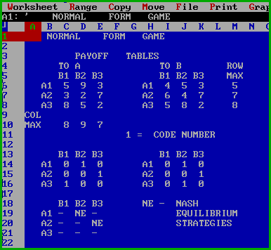
Inspection of this table reveals, by trial and error, that there are two strategy pairs, (A1,B2) and (A2,B3) that satisfy the Nash equilibrium condition that each player's strategy is a best response to the other's.To model this game on a spreadsheet it is necessary to use the data from Figure 1 to create two separate payoff tables for A and B, as shown in the top section of Figure 2.

Figure 2: Normal Form Game
Layout and Labelling
All columns should be reduced to width 3 and labels entered as shown in Figure 2.Data
Enter the payoff data given for A in Figure 1 into cells C6 to E8 and the payoff data for B into cells I6 to K8.Formulae and Calculations
To find A's best response to each of B's strategies we need to find the column maximums for A's payoff table.Enter @MAX(C6.C8) in cell C10.
Copy this formula from C10 to cells D10 and E10.
The column maximum indicates the payoff to A when it chooses its best response to B's strategy corresponding to that column.
To find B's best response to each of A's strategies we need to find row maximums for B's payoff table.
Enter @MAX(I6.K6) in cell M6 and then copy to M7 and M8.
We now need to find out which, if any, pairs of strategies correspond to both a column maximum for A's payoff table and a row maximum for B's payoff table. This is done by first identifying which cells in the payoff tables contain the column and row maxi mums, respectively, and putting the number 1 in these cells.
This identifying code number is put in cell G11.
A new set of payoff matrices is created in rows 14 to 16.
In cell C14 enter @IF(C6=C$10,$G$11,$A$11).
This will cause 1 to appear in C14 if C6 equals the column maximum in C10 and 0, from A11, to appear if it is not.
This formula can now be copied from C14 to C15 and C16 as the row 10 is anchored with the $.
In this example the code 1 appears in C16 as strategy A3 is A's best response if B plays B1.
To code A's best responses to B2 and B3 copy from the three cells C14.C16 to the column sections commencing D14 and E14.
To code B's best responses to each of A's strategies we need to mark up which cells in B's payoff matrix correspond to the row maximums in cells M6 to M8.
In cell I14 enter @IF(I5=$M5,$G$11,$A$11)
Note that this time it is the column M which is $ anchored.
Copy the formula from I14 to J14 and K14, then copy from the three cells I14.K14 to the row sections commencing I15 and I16.
If a pair of strategies is a Nash equilibrium each player will be receiving the maximum payoff possible, given the other player's strategy.
This means that there will be a 1 in both of the coded payoff matrices for this strategy combination. Any such Nash equilibrium strategy pairs in the final matrix can be coded "NE" in a single matrix of strategy combinations by adding the two matrices already coded and finding cells whose value is 2, i.e. where the strategy combination is both a column maximum for A and a row maximum for B.
In cell C19 enter the formula @IF(+C14+I14>$G$11,$H$19,$I$19).
This will display the code NE from cell H19 when the value in C19 is greater than the value 1 in G11, i.e. when it equals 2. The dash in I19 is displayed when C19 has the value less than 2. Copy this formula from C19 to the rest of the cells in the matrix C19.E21.
The two strategy combinations coded NE in this matrix are the same as those found by the trial and error visual inspection method for Figure 1.
In this simple example the time saved by using a spreadsheet may not be all that great but from a student's viewpoint it is a good means of checking that they have in fact found all the Nash Equilibrium solutions.
More complex games can be solved by using the basic principles developed here to construct spreadsheets to deal with payoff tables with larger numbers of rows and columns.
Extensive form games (Game Trees) -
Oligopoly Entry Game
A basic introduction to game trees and their application to
oligopoly entry is provided by Katz and Rosen (1994).Consider the following problem where there are two players who decide their actions sequentially. Firm N is considering entering a market where firm I is currently the monopoly incumbent. The incumbent I has two possible actions which it can use to try to deter entrants: High output or Low output. It can wait until N has made its decision to enter or stay out before deciding on High or Low output.
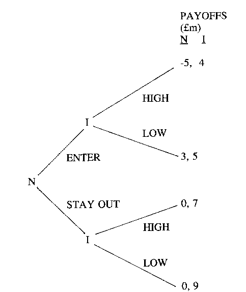
If N does enter the payoffs (in śm profit) to N and I, respectively, will be (-5,4) if I decides on High output, and drives down the price to scare off N, and (3,5) if I responds with Low output and lets N into the market. On the other hand, if N stays out the payoffs will be (0,7) if I decides on high output and (0,9) if it decides on Low output.
Each firm has full information about the payoffs resulting from each combination of actions.The game tree illustrating this problem is shown in Figure 3.

Figure 3: Payoffs from oligopoly game with full information
Firm N's strategy set is simply the set of its two possible actions, Enter or Stay Out. Firm I has a larger set of strategies as it can relate its action choice to action already taken by firm N.For example a possible strategy may be "play Low output if I enters, play High output if I stays out".
The solution to this game can be deduced from Figure 3 as follows:
If N enters then I's best action is to play Low output, giving a payoff of Ł5m, as opposed to Ł4m if it played High output. Thus N's payoff would be Ł3m.
If N stays out then I will maximise its payoff by playing Low output, yielding Ł9m. As N does not enter the market its payoff is zero.
Thus, in this example, N will choose Enter as it yields N the highest payoffs (ś3m) when I has responded with its choice of output level. The solution is thus: N enters, I produces Low output and payoffs are Ł3m, Ł5m.
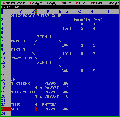
A spreadsheet model that will solve this type of problem is shown in Figure 4 and constructed as described below.

Figure 4: Spreadsheet Model
Layout and Labelling
Columns B,C and E reduced to width 1.Columns F,G and H reduced to width 4.
Column A increased to width 9.
Labels in rows 1 to 4 are enterd as shown in Figure 4.
Note that the labelling apostophe has to be enterd before the oblique lines (e.g. '/ entered in cell C7). Labels for lettering in rows 15 to 24 are as shown in Figure 4 except for cells F17, F19, D22 and F23 which are left empty for formulae.
Data
The payoff data given in the question for the four possible combinations of actions is entered in the four pairs of cells G4 and H4, G8 and H8, G10 and H10, G14 and H14.
Formulae and calculations
In cell F17 we wish to display I's output action when N enters. This will correspond to the higher of the values in cells H4 and H8.To do this enter the formula @IF(H4>H8,F4,F8) in cell F17.
To display the corresponding payoff to N enter in cell F18 the formula @IF(H4>H8,G4,G8).
To display I's action when N stays out enter in cell F19 the formula @IF(H10>H14,F10,F14).
N's payoff is displayed by placing in cell F20 the formula @IF(H10>H14,G10,G14).
Firms N's decision to enter or stay out now depends on the values of its payoff in cells F18 and F20, respectively.
To display the action taken by N place in cell D22 the formula @IF(F18>F20,A7,A11).
To display the action by I when N plays the strategy shown in D22 enter the following in cell F23 @IF(F18>F20,A17,A19).
As well as being used to check the solution to simple games in this format the principles used to develop this spreadsheet can be used to formulate templates to solve more complex game trees, as the following section shows.
Commitment and Incomplete Information
Assume that the incumbent I in the example above has the option of investing in a larger size plant to demonstrate its commitment to driving out potential rivals in a price war. If it does build a larger plant the respective payoffs to N and I will be:(-5,7) if N enters and I chooses High output
(3,4) if N enters and I chooses Low output
(0,8) if N stays out and I chooses High output
(0,5) if N stays out and I chooses low output.
Also assume that N is not sure whether or not I has invested in the larger plant when it makes its decision to enter or stay out, i.e. there is incomplete information.
If N believes believes there is a 0.5 probability that I still has the original size plant, and payoffs are still as in the previous example, the question is "will N enter or stay out?"
To solve this game of incomplete information we need to look at how N calculates the expected value of its payoffs. From the previous example we know the N's predicted payoff will be Ł3m when I has the original small plant. From the new set of payoff figures we can see that if I builds the larger plant then:
- if N enters, I's best action is High output giving I a Ł7m payoff with N facing a loss of Ł5m, and
- if N stays out, I's best action is High again, giving I an Ł8m payoff with N obviously receiving nothing as it produces nothing.
If it is assumed that N believes I still has the original small plant with a probability p then its expected payoffs (in śm) are:
Enter: 3p + (1-p)(-5) = 8p - 5
Stay out: Zero (since there is no production)
Thus N will enter if 8p - 5 > 0 or p > 5/8
Thus with p = 0.5 the solution to this game is that N will enter.
Now let us construct a spreadsheet that can be used to derive this solution. It is quicker to amend the template constructed for the basic Oligopoly Entry game as in Figure 4 than to start again from scratch.
Layout and Labelling
Load the template saved for Figure 4. Before anything else is done use the /FS command to save it back onto disk under a new filename. This should stop the new template overwriting the original file.Erase the titles in row 1. Delete rows 16 to 23. Insert three new colums to the left of the original column A. Reduce the width of columns B and C to 1. Increase the width of column D to 10.
Copy the section of the template now in cells D4.K14 to cells D16.K26. Now enter lables in the rest of the template as shown in Figure 5. Note that the vertical lines A11.A14 and A16.A19 require the labelling apostrophe. Right justify labels in cells A11.A14 and A16.A19. Centre justify label in A15. The script in cells G32, G36 and G42 will display outputs produced by formulae and so these cells should be left empty at this stage.
Data Entry
Since this example has the same payoff figures as in Figure 4 for the small plant situation no new data has to be entered in the top half of this game tree. As this has now been reproduced in the bottom of the game tree by the copy command these numbers need to be changed to reflect the new set of payoffs when I has a large plant.Enter 0.5 in cell I29. This is what N believes to be the probability that I still has the original small plant.
Formulae and calculations
We need to find the expected payoffs to N for the two possible scenarios:
- I still has the original small plant
- I has built a new large plant.
If I has built a new large plant its response to N entering can be shown in cell G36 by using the formula @IF(K16>K20,I16,I20) and the resulting payoff to N is shown in cell G37 using @IF(K16>K20,J16,J20).
N's expected payoff if it enters can now be calculated in cell G40 using the formula +G33*I29+(1-I29)*G37.
Since the payoff from not entering is always zero, firm N will enter if this expected value of the payoff from entering (held in G40) is a positive number. The outcome of this decision is diplayed when @IF(G40>0,D7,D11) is entered in cell G42.
References
- Bierman H S and Fernadez L (1993) Game Theory with Economic Applications. Addison-Wesley, Mass.
- Gibbons R (1992) A Primer in Game Theory. Harvester-Wheatsheaf, Hemel Hempstead.
- Hawdon D and Anderson J (1992) Games for Economic Modelling, in Anderson J and Hawdon D (eds) Enterprising Uses of Computer Resources. Department of Economics, University of Surrey.
- Katz M L and Rosen J S (1994) Microeconomics, 2nd ed. Irwin, Illinois.
|
What's Related: · Other articles on the use of spreadsheets in teaching economics |

