Volume 17, 2005
Simple Cellular Automata on a Spreadsheet
- Chris Hand
- Post-Doctoral Researcher, Kingston University, Kingston-upon-Thames
Abstract
Cellular Automata (CA) can be used to illustrate how macro-level order can arise from micro-level interactions. Although it is possible to run simple CAs using pencil and paper, a computer is better able to keep track of all the interactions. This paper illustrates how simple CAs can be run on a spreadsheet, using the diffusion of a product innovation as an example.
Introduction
This paper demonstrates the implementation of a cellular automaton (CA) on a spreadsheet. CA models provide a clear demonstration of a phenomenon known as emergence – order arising from the interaction of agents rather than as the result of centralised control. Perhaps the best-known application of a cellular automata-type model in the social sciences is Thomas Schelling’s model of racial segregation (Schelling, 1971), although CAs may also be used to model the diffusion of innovations or the spread of rumours, to name just two applications. Gaylord and D’Andria (1998), Hegselmann and Flache (1998) and Gilbert and Troitzsch (1999) discuss further applications of CAs in the social sciences, while Torrens (2000) reviews the use of CAs in the study of urban systems.
What are cellular automata?
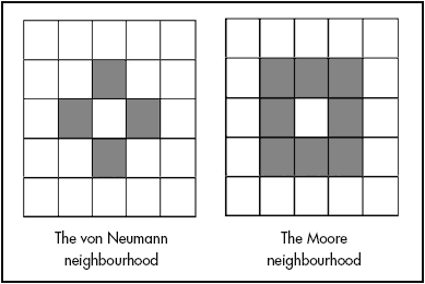
Cellular automata are dynamic models of local interactions between cells on a regular d-dimensional grid. Each cell may be in one of a predetermined number of states (e.g. on or off, alive or dead). As the simulation progresses step by step, the state that a particular cell is in depends on its state in the previous period and the state of its immediate neighbours according to a simple rule. This rule is applied to all cells on the grid. The neighbouring cells are often defined as the eight cells surrounding the cell, known as a Moore neighbourhood, or as the cells directly above, below, to the left and to the right of the cell, known as the von Neumann neighbourhood (see Gilbert and Troitzsch, 1999). The von Neumann and Moore neighbourhoods are shown in Figure 1.
Figure 1. CA neighbourhoods.
One of the best-known applications of a cellular automaton is the Game of Life (see, for example, Waldrop, 1992; Holland, 1998). In the Game of Life, a cell survives only if two or three of its neighbours are alive. If there are more or fewer neighbours alive then the cell dies, from either over-crowding or loneliness. A dead cell is brought back to life if it has three living neighbours. From these simple rules, myriad ever-changing patterns emerge.(note 1) Whilst it certainly possible to conduct small simulations by hand – as Casti (1994) recounts, Schelling’s initial runs of the segregation model used a draughtboard – it is far easier to use a computer. It is not always necessary to write a computer program to implement a CA. CA models can also be implemented using software packages such as Mathematica (see Gaylord and D’Andria, 1998) and StarLogo (Resnick, 1997). However, simple CAs (i.e. those where a cell can be in one of two states) can be modelled on a spreadsheet. A spreadsheet model displays the inner workings of the CA and gives the modeller direct control over the model, without the need for programming skills.
A general example: the diffusion model
Cellular automata are increasingly being used in economics, especially in urban/spatial economic models. Macken and Randall (1994) employed the concept to develop a ‘Privatisation and Nationalisation’ module in the computer-aided learning package WinEcon. Moreover, CAs can be applied to any situation involving local interaction, such as the diffusion of information or rumours, models of opinion formation or the adoption of new technologies. This section demonstrates a diffusion model on a 10 x 10 grid. Each cell represents an individual who may be in one of two states: they may have heard of the new product (these cells are coloured black) and they may not have (these cells are coloured white). An individual cell turns black if one of its four von Neumann neighbours is coloured black. This rule can be implemented using Excel’s ‘if’ function.
To begin, select a 10 x 10 grid of cells to be the initial state of the CA. The cells in this case represent economic agents. A cell contains the value 1 if an agent has adopted a new innovation and contains 0 otherwise. The ‘if’ function encapsulating the CA rule is entered in each cell of an identical grid immediately below the first grid. In general, for a given cell e, with neighbours a, b, c and d, the ‘if’ function is:
=if(ai+bi+ci+di>=1,1,ei)
or equivalently
=if(ai=1,1,if(bi=1,1, if(ci=1,1, if(di=1,1,ei))))
where the subscript i refers to the state of the cell in the initial grid. For cells in the centre of the grid, this is easy to implement. However, a little more care needs to be taken with cells in the top and bottom rows and extreme left-and right-hand columns. Neighbourhoods of cells in the top and bottom rows and in the extreme left- and right-hand columns ‘wrap around’ the grid, so for a cell in the top row, its ‘northern’ neighbour will appear in the bottom row of the grid. Similarly, the ‘western’ neighbour of a cell in the extreme left-hand column of the grid is in the extreme right-hand column, as shown in Figure 2.
Figure 2: Wraparound CA neighbourhoods.
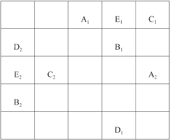
The second grid (containing the formulae) shows the state of the CA after the first iteration. Further iterations can be obtained by copying the grid and pasting down the page. As long as the same spacing between the grids is maintained, the formulae will automatically update.
It is not easy to spot patterns in a range of 0s and 1s. To ease matters, the ‘if’ function can be used again to create a grid of blank and filled cells using the following formula:
=if(a1=1,“#”,“ ”)
Figure 3 shows the initial set-up for the CA.
Figure 3: Setting up the cellular automaton.
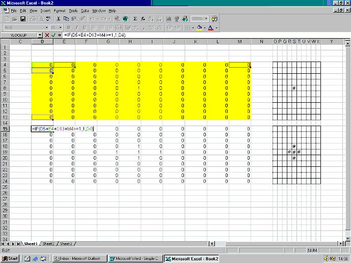
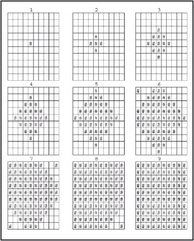
The initial state of the CA is shown in cells D4 to M13. In this example, only 1 of the 100 agents has purchased the new good. The ‘if’ functions containing the rules of the CA are entered in cells D15 to M24. Alongside these two blocks of cells are two more grids which display the same information, using a # to represent 1 and a blank to represent 0, according to the ‘if’ function described in equation (3). To see how the new innovation spreads, the formulae in cells D15 to M24 can be copied and pasted down the page, with an empty row between each copy. Without this empty row, the formulae will not refer to the correct cells. In this example, the innovation diffuses across the whole grid in only nine iterations, as shown in Figure 4.
Figure 4: The diffusion model.
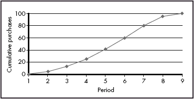
The standard product life cycle/diffusion model would suggest that a plot of cumulative sales should trace out a curve like the logistic curve (see, for example, Bass, 1969). A plot of cumulative purchases (i.e. the number of cells containing 1s in each period) derived from the CA simulation also produces a logistic-like curve, as shown in Figure 5.
Figure 5: Cumulative purchases in the CA simulation.
Extensions to the model
The deterministic model presented above is unrealistic, as once one agent has bought the new item, all the others will do so too. The model can be extended by introducing a stochastic element into the way a cell is affected by its neighbours. In this model, a blank cell becomes filled with a given probability if at least one of its neighbours is filled. This is achieved on a spreadsheet using Excel’s random number generator to create a random number between 0 and 1 for each agent (each cell). A filled cell will influence its neighbour if the random value assigned to it is less than the level of probability specified. The CA rule then becomes:
=if(ai*ra>p,1,if(bi*rb>p,1,if(ci*rc>p,1,if(di*rd>p,1,ei))))
where rj(j=a,b,c,d) is a random number between 0 and 1 associated with cell j and p is 1 minus the given probability. Defining p as 1 minus the given probability allows the formula to be written as above. If the given probability level were entered directly into the formula =if(a*ra<p,1…), Excel would regard all blank cells (given the value 0) as meeting this criteria and return a value of 1 for every cell. The agent represented by cell e will adopt the new innovation if at least one neighbouring cell has adopted and the random number associated with that neighbour exceeds the chosen probability level p. The screen grab below shows this new CA, with the initial state of the grid in cells E5..N14, the formulae entered in cells E16..N25 and the random numbers entered in cells P16..Y25.
Figure 6: Modified CA diffusion model.
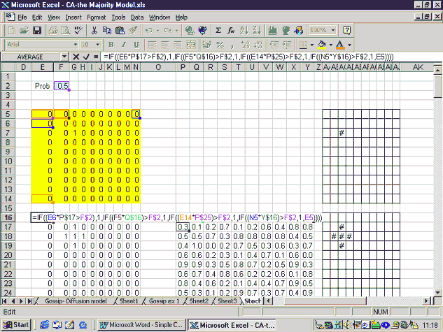
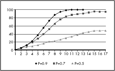
As set up above, once the formulae have been entered, the effect of a change in the probability can be easily found. Note that the probability that a blank cell becomes filled is 1 minus the probability level entered in cell F2. For sufficiently high probability (sufficiently low values entered in cell F2), the plot of cumulative adoption resembles the logistic plot expected in the product lifecycle model, as shown in Figure 7. It should be noted, however, that these plots were obtained from a CA model with the same random number grid and initial distribution of adopters in period 1.
Figure 7: The extent of diffusion under selected probabilities.
In the stochastic diffusion model, it is not guaranteed that a new innovation will diffuse across all agents. This can be demonstrated by holding P constant and running the simulation a number of times using a different initial state for each run.
Running the simulation ten times with a 70% probability that a blank cell becomes filled if one of its neighbours is filled, and with a different cell given the value of 1 in the initial grid in each run, yielded the results shown in Figure 8.
Figure 8: The effect of different starting configurations (P = 70%).
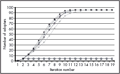
In this example, as long as there are a sufficient number of early adopters, the innovation will diffuse across most of the grid. Where this early support is not achieved, adoption is restricted to a few or in some cases only one agent on the grid.
Conclusion
CA models may be used to demonstrate how the characteristic graphs of the product life cycle emerge from the behaviour of the individual agents and how the model still holds if a cell is influenced by its neighbours with a sufficiently high probability. This is, however, only one potential application of cellular automata in economics and in other social sciences. The examples described by Gilbert and Troitzsch (1999), such as the Game of Life and the majority model, can be reproduced on a spreadsheet with equal ease (see appendix). An advantage of using a spreadsheet to investigate cellular automata is that the workings of the model are made explicit. The assumptions employed and the relationship between cells are encapsulated in the formulae used. Spreadsheet CA models are limited to relatively simple examples, but they give the same amount of control over the model as a CA program written in, for example, Visual Basic, without the need for programming skills. Furthermore, these CA models can provide an easy introduction to the notion that order can emerge in a system of interacting agents, such as a market, purely as a result of dynamic interactions. Spreadsheet CA models could thus be used as a simple introduction to agent-based models and modelling in economics, as advocated recently by Ormerod (2003).
Appendix: The majority model
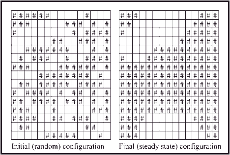
In the majority model, a cell will change from white to black if the majority of its neighbours are black. One could see this model as a variation on the diffusion model; rather than adopting the new product when one neighbour has adopted it, each agent waits until the majority of its neighbours have adopted it. The spreadsheet models show that even with modest preferences (i.e. the cell changing to match just over half its neighbours), the cells form distinct solid blocks. This is reminiscent of Schelling’s finding that communities can become racially segregated even when each agent has only a mild preference for neighbours of his/her own race. The version of the majority model shown here employs the Moore neighbourhood (8 neighbours) rather than the von Neumann neighbourhood employed in the examples above. Each cell can be in one of two initial states, denoted by 1 and 0. If the sum of each cell’s neighbours is greater than or equal to 5, the cell turns to (or remains) in state 1, whereas if the sum is less than or equal to 4, the cell changes to (or remains) in state 0. This rule can be implemented with Excel’s ‘if’ function, as in the diffusion model. A screen grab of the majority model is shown in Figure A1.
The initial state for each cell is shown in cells B2–P16 and the ‘if’ formulae are entered in cells B18–P32, ready to be copied down the page. This particular example reaches its steady state after 10 iterations. The initial and final configurations of the cells are shown in Figure A2.
Figure A1: The Majority Model
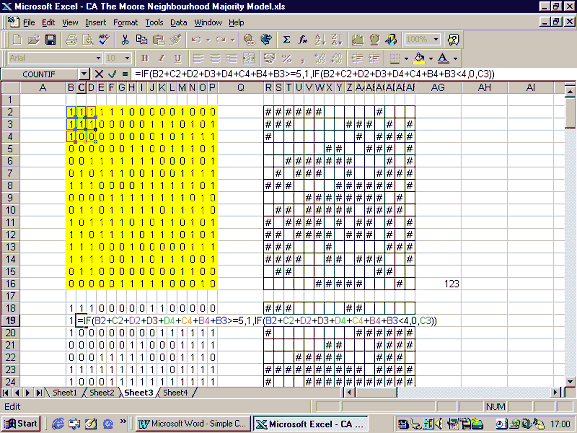
Figure A2: The Majority Model
Note
For a demonstration of the Game of Life, see http://www.math.com/students/wonders/life/life.html .
References
Bass, F. M. (1969) ‘A new product growth model for consumer durables’, Management Science, 15, pp. 215–27.
Casti, J. (1994) Complexification, London: Abacus.
Gaylord, R. J. and D’Andria, L. J. (1998) Simulating Society: A Mathematical Toolkit for Modelling Socioeconomic Behaviour, Berlin: TELOS Springer-Verlag.
Gilbert, N. and Troitzsch, K. G. (1999) Simulation for the Social Scientist, Buckingham: Open University Press
Hegselmann, R. and Flache, A. (1998) ‘Understanding complex social dynamics: a plea for cellular automata based modelling’, Journal of Artificial Societies and Social Simulation, 1(3), [online] available from: http://www.soc.surrey.ac.uk/JASSS/1/3/1.html .
Holland, J. H. (1998) Emergence, from Chaos to Order, Oxford: Oxford University Press.
Macken, K. and Randall, K. (1994) ‘Teaching and learning economics using cellular automata in Asymmetrix Toolbox’, Computers in Higher Education Review, 8(3), p. 12.
Ormerod, P. (2003) ‘Turning the tide: bringing economics teaching into the twenty-first century’, International Review of Economics Education, vol. 1, [online] available at http://www.economicsnetwork.ac.uk/iree/i1/ormerod.htm .
Resnick, M. (1997) Turtles, Termites and Traffic Jams: Explorations in Massively Parallel Microworlds, Cambridge, MA: MIT Press.
Schelling, T. C. (1971) ‘Dynamic models of segregation’, Journal of Mathematical Sociology, 1, pp. 143–86.
Torrens, P. M. (2000) ‘How cellular models of urban systems work (1. theory)’, Centre for Advanced Spatial Analysis (CASA) Working Paper no. 28, University College London.
Waldrop, M. (1992) Complexity, the Emerging Science at the Edge of Order and Chaos, London: Penguin.
Contact details
Chris Hand, Post-Doctoral Researcher
Faculty of Business
Kingston University
Kingston-upon-Thames
Surrey KT2 7LB
Email: c.hand@kingston.ac.uk

