Volume 15, Issue 1, 2002

TK Solver Release 4. UTS Software
- Ronald Shone
- University of Stirling
Installation
Installation is quick and easy. If the standalone version is purchased, the instructions that come with the package, which refer only to networks can be ignored. There is no indication of what to do if you have an existing version, but this should be uninstalled first before installing version 4 (There is little point in having both versions on the same machine). All earlier versions's files can be loaded with no difficulty into version 4.
What is TK Solver?
TK Solver is a package for solving numerical equations - whether linear or nonlinear, or single or multiple equations - up to 32,000 in all! If you consider the equations as representing a "model", then the model can be entered in any order, which often means entering them as an economist would naturally think about the model: a demand equation, a supply equation and an equilibrium condition, to give the simplest. There is no need to arrange the variables in any specific order, or write the equations as the endogenous variables in terms of the exogenous variables. All that is required is that there are enough equations to solve for the endogenous variables of the model. This is especially important if the model is nonlinear or dynamic. Of particular importance is the fact that the model does not need to have the endogenous variable fixed immutably. When, for instance, undertaking some question of policy, it may be necessary to declare (say) government spending as an endogenous variable and income as some target level (which is then exogenous). It is this flexibility of model construction that is the essential strength of TK Solver.
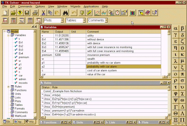
To see this in action, consider the moral hazard problem illustrated in Figure 1, from Nicholson's Microeconomic Theory. Three windows are displayed: the top right, which sets out the equations of the model; the bottom right, which lists all the variables of the model; and the left navigation window which lists the various sheets which are used to set out the whole model in TK Solver. Notice also how the navigation window on the left lists the variables of the model. This model in particular is nonlinear, because the utility function used is attempting to capture risk aversion. Besides the value of utility for initial wealth, the model is solving for various expected levels of utility depending on whether the individual does or does not install a theft device in his or her car and whether they choose to take out full insurance cover with or without being monitored by the insurance company. For this version of the model the probabilities are input values. When solving the model TK Solver checks the integrity of the model, and will supply information on aspects such as inconsistent equations, over-determined equations, etc. This method of solving is referred to as forward solving.

Figure 1
But suppose you wanted to know what the probability of theft would have to be in order for the expected utility under full cover insurance with monitoring to be the same as the level under simply installing a theft device. In this instance you need to include in the set of rules the condition Ev4 = Ev2, and change p2 from being an input value to being an output value. Then re-solve. However, because Ev4 = Ev2 has the probability on both sides of the equation, it is necessary to invoke the iterative solver by supplying a guess value for p2 (see the later section on solving). This is quite straightforward to do, and gives the probability just over 0.9. In fact, many such questions can be asked of a model, and often all that is required is to change input values and output values appropriately, sometimes including some additional rules where necessary. This is referred to as backward solving. It is this flexibility of doing forward and backward solving that is one of TK Solver's main features.
Sheets
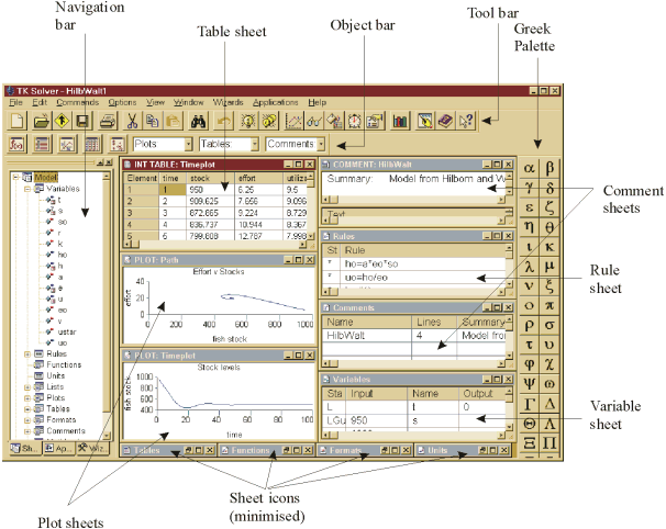
Figure 1 illustrated just two of the sheets used by TK Solver to set out a model and its results. There are nine sheets in all: rules; variables; tables; plots; functions; formats; lists; comments and units. Each sheet has its own window. Although this seems excessive for a small model, this is not so for a large model. This use of sheets allows the model to be handled logically and allows an uncluttered screen to be worked on. In simple terms, the model is seen in modular form, and only the sheets of interest to the user need to be displayed at any one time. A model with multiple windows being displayed simultaneously is illustrated in Figure 2, where the main features of the display are highlighted.

Figure 2
The MathLook window was a new innovation in version 3.32. This has been much improved in version 4. TK Solver now has the following.
- Dynamic links with other sheets in the model.
- Known and unknown values distinguished by colour.
- Object alignment.
- The facility to add text, pictures and page breaks.
- A MathLook toolbar.
- Automatic updates of data and plots in response to changes.
The MathLook window is also the place where formulas in Excel can be checked because they display formulae more closely to their mathematical counterpart rather than a single string with endless nested brackets. As we shall note later, the link with Excel is a particularly new innovation in version 4. Useful as the MathLook window is, it is not without its own problems, which are referred to later in this review.
Solving
Obviously, solving is the main use of TK Solver. For simple systems the programme solves the model directly, so long as there are enough consistent equations to do so. From an economic modelling point of view, we would see the output variables as the endogenous variables of the model, and all input variables as exogenous. All parameter values must also have input values for the model to be solved. Direct solving, in particular is invoked if the same variable does not appear on both sides of the equal sign. If the same variable does appear on both sides of the equation, for instance solving for x in the formula x = exp(a*x) with a a known constant, then the programme uses an iterative solver. Iterative solving is also used for solving nonlinear models. To employ the iterative solver, it is necessary to supply guess values for one or more of the variables, declaring them as guess values in the status column (see the status column highlighted in Figure 2). For most problems the iterative solver will converge on a solution very rapidly. Two issues are important here. First, for nonlinear models there can be more than one solution. Second, because of the algorithm used, or because of the nature of the model itself, the system may tend to a cycle before a solution is found (Discrete systems are more prone to such cycles than continuous ones!). In either case, it is necessary to supply "good" initial values for the guess, and these will have a bearing on whether one or other of these problems arises.
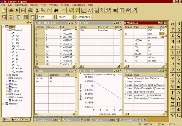
List solving is a particularly useful solver. At its simplest it is useful for plotting functions. If for example you have y = f(x), then one can readily construct a list of values of x over some specified range and obtain the value of y resulting. Then it is a simple matter of plotting y against x. It is no more difficult if y is the outcome of some model that is solved directly for each value of x, with the resulting value of y being plotted against each value of x. The fact that y can be the output of some model is where TK Solver wins over Excel. We can illustrate list solving utilising the example in Figure 1. Suppose we wish to consider the expected utility for various values of monitoring costs. Suppose we allow monitoring costs to have the range 0 to 20 in step values of 2. We note that monitoring costs (denoted mcosts) only occur in Ev4. So if mcosts are declared as an input list, then Ev4 will need to be declared as an output list. Of course, when the mcosts equal 10, then this is the result we have in Figure 1, but now this is only one of the output values. In Figure 3 we plot the expected utility against the monitoring costs and also show the table of values. The plot and the table where created by the list wizard. Although a bit of a contrived example, it does illustrate the list solver in operation.

Figure 3
But list solving is particularly important when considering dynamic systems - especially nonlinear dynamic systems. A dynamic model often comprises a set of simultaneous equations, either linear or nonlinear or a mixture of the two. The simple cobweb model of demand and supply is a case in point. In such a model expected prices are expressed as some function of past prices. It may simply be the price in the previous period, or some weighted average of the past price and the past-expected price. Whatever the expression for expected prices, the model needs to be solved simultaneously from some starting price, and this needs to be done for each time period. Although spreadsheets can readily be used for simple models in which a reduced form for the current price can be found in terms of actual past prices, if the equations are nonlinear, this may not be the case. In this instance spreadsheets are not much use. This is where list solving really pays off. From the initial price, which is a given input value, time is declared as a list and price is simply the solution to the model in each time period, which is itself a list (output).
Another list solving feature is block solving. This solves for a selected group of list elements. In economic models this would be useful if the model is of a recursive nature.
Wizards
Wizards have now become commonplace in software programming - and nothing to do with Harry Potter! There are seven wizards included with TK Solver 4: units import; object sorting; plotting; list solving, model printing, object units summary and global units swap. Some are new to version 4 while others are improvements over earlier versions. Since list solving is not the easiest of the solvers, it is useful to have a list-solving wizard. This wizard was invoked to create the plot and table in Figure 3. Model printing is also quite useful, but there are some difficulties with printing Greek letters (see my problems with the package later in this review.)
A summary of some other new features
Three cosmetic changes have been introduced; the navigation bar, which is the most important, smart editing, and the (now common) use of the right click of the mouse button for context sensitive editing. The navigation bar, seen in the left window in Figure 1, summarises the whole model. But it is also useful for opening up individual sheets when required. Smart editing simply means that the programme keeps track of information typed in and will suggest test as you type. Not a useful facility in my view. The context sensitive right click is far more useful, especially for inputting built-in functions. Also included now is Find, Replace and Go-to commands along with Find in Model. Obviously these are more useful the larger the model is and/or the more sheets one uses to set out the model. There is, however, a problem of finding Greek variables!
Plotting has been much improved. It was fairly basic in earlier editions and allowed very little in the way of annotations. Now legends and annotations can be included. Plots can be saved as GIF or JPEG images, which are useful for inserting into other programmes or the Web. Furthermore, copy and pasting of plots preserves the resolution and so the printing of plots in other programmes is now better.
A whole model, a single window or part of a window can now be exported in HTML format. Exporting a whole model must be done to its own folder, which contains no other HTML file. The results of such an export produce each of the sheets one after the other on the Web site. All 9 sheets plus the MathLook window appear on the Web, as do the subsheets. This means each variable and parameter, which contains its own subsheet, is included. In a large model this can be too much detail. However, it is possible to export just a subset that contains the essential information. Since the Web is becoming one of the main means of displaying and communicating information, this new facility is quite important.
Other new elements, not so much features, are built-in functions. It is impossible to cover this topic in a short review, but the area that will be of interest to the economist is that of differential equations. Differential equations are obviously continuous equations. Solution methods are usually numerical, however, especially where no obvious solution method is known. In earlier editions these were part of the library, but in version 4 they have been included in the set of built-in functions. It may be worth mentioning in passing that TK Solver also allows the user to define their own functions. Also new to version 4, and included in the library, are solutions to financial models. It must be stressed that these are very basic and are no more than solving for interest payments, loans, annuities, and the like.
Using TK Solver with Excel
The link between TK Solver and Excel is particularly new to this release. The domination of Microsoft is becoming quite evident in seeing mathematical programmes linking to Excel. Mathematica, Maple and now TK Solver all link to Microsoft Excel. Excel is particularly good at displaying data but not so good at solving models. What has been happening over the last few years is to use the mathematical programmes to do all the solving and in-depth calculations and then to display the results in Excel. In effect, Excel becomes a front-end and the maths programmes become the engine or kernel. The user does not necessarily have to know what goes on behind the scenes. Of course, this facility is not of interest to everyone.
Installing the TK Solver-Excel toolkit is quite straight forward and once contained in the add-ins tools one sees a new item called MathLook, which itself has five items: Show Mathlook, Load Model, Update TK Solver, Show TK Solver and Run TK Solver Wizard. These can also be placed on the toolbar. The Show MathLook opens the MathLook for Excel dialog box; Load Model opens a dialog for choosing a particular TK model to load into the TK Solver add-in; Update TK Solver recalculates the TK Solver model in background with updated inputs from the Excel worksheet; Show TK solver opens TK Solver directly from Excel; and Run TK Solver Wizard starts this wizard which links an existing TK model with the current worksheet.
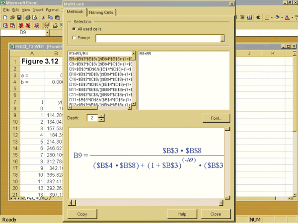
The MathLook is quite useful for anyone using many formulas in their spreadsheets. The upper left hand window lists the cells and their formulas (only cells with formulas are displayed in this window). The upper right hand window displays formulas for additional cells in the main formula. In the bottom window, the equation is displayed in conventional mathematical style, as shown in Figure 4. Another nice facility is the "naming cells" tab, which displays the formulas using cell addresses - both relative and absolute.

Figure 4
Following the example in the manual for linking TK Solver and Excel was not easy for anyone not familiar with macros or Visual Basic Editing. It also gives instructions to copy the information between the two dotted lines, but then in Step 4 asks the user to find the "Workbook_Open()" procedure. This, however, is not contained between the two dotted lines. If this is necessary, then why not place it there? I strongly suspect that anyone not familiar with the Visual Basic Editor will refrain from using the TK Solver - Excel link. They will likely choose to use one or the other package and transfer the relevant information across, which is not that difficult.
Problems encountered
The first problem I encountered was the impossibility of searching or find/replace/goto for any Greek character. l for instance was listed in the navigation window as �. Another problem encountered with the use of Greek letters for variables is in the printing and displaying of the model. The Greek is displayed OK in the MathLook window, but if the model is printed using the print wizard, the variable sheet cannot cope with the Greek letters. The Getting started book simply says use a Greek language script font. But which true type font satisfies this? Is the user expected to find one by trial and error? Oddly, the problem does not occur when printing the variable sheet, since Arial (with a Greek extension) can be chosen. This option does not appear when using the Print Wizard. There is, however, no difficulty when pasting as a picture in Word. There seems a general lack of thought concerning the Greek palette. An earlier version needed a patch and now the find/replace/goto does not integrate with it.
I had a number of problems with the MathLook window. The first problem was with the insertion of a page break. They apparently occur not at the end of some insertion point - although I could never establish where my insertion point was actually located! The manual refers to after the cursor position, but then I found no cursor shown in the MathLook window! For this reason I also had problems inserting elements of the model suitably in the MathLook window, sometimes they overlaid each other, while at other times they almost appeared at some random spot! A second problem encountered with the printing of the MathLook window was the occasional missing bracket at the end of an equation.
Another problem found was with the currency conversion. This is new to this edition. The default is converting from dollars into twelve other currencies, including the euro. But when using the import units wizard and setting input to be the British Pound, the units imported where all to do with the dollar! What I was expecting is units to be from the British Pound to the other twelve currencies. No matter what currency I chose in the left panel I always had conversions from dollars into the other currencies. Is this yet another example of programmes defaulting to whatever is the US convention?
The TK Solver-Excel toolkit is not without problems. The first I encountered was in situations where my spreadsheet had thousands of data entries - all doing similar calculations and so all I really needed to check was the first 10-20 lines. Although the MathLook does come with the facility to choose a range of cells, you can only do this once the MathLook window is open, but to open it it defaults to all used cells. What this suggests is that the MathLook facility be used at the early stages when seeing and checking the formulas you enter. There need not even be thousands of data for the programme to take some time to display the MathLook window with its default to all used cells. A spreadsheet of just 25x5 took an inordinately long time to display the MathLook window, as did some spreadsheets of much smaller dimension. It is not possible to do anything else while this is happening. It would have been better to set the programme up in such a way that the user first blocked the cells and only these would be displayed in the MathLook window.
A second problem, also to do with the MathLook window, was that it could not be resized. It required the full height of my screen. But I place my office toolbar at the top rather than the side, which meant part of the MathLook window containing the typical three windows control buttons on the top right was obscured. Moving the window down to display these meant the control buttons for copy, help and close disappeared off the bottom of the screen! It would have been better to allow this window to be resized.
A third problem arose when following the model in the user manual for linking Excel and TK Solver. This is the simple loan formula. When following the instructions, it says to save the model (p.13-28) but this could not in fact be done and since it could not be done, there was no way to link the model with the worksheet! The model in TK Solver needs to be created and saved first.
Conclusion
TK Solver remains a specialist problem-solving package. What it does, it does well. However, the enhancements need improving. For those individuals familiar with earlier version of the package, the enhancements will be welcome. Will they attract many new users? I suspect not. Even so, the package does deserve a much wider use. But for this to occur, the suppliers need to illustrate its applicability outside the area of engineering.

