

by Siem Jan Koopman, Andrew C. Harvey, Jurgen A. Doornik and Neil Shephard
STAMP 6.0 is the new Windows version of the program designed for modelling and forecasting time series using the structural time series approach. With this approach one assumes that a series (or a group of series, since multivariate as well as univariate models can be constructed) can be represented in terms of a set of additive unobservable components which have natural interpretations: - trend, cycle, seasonal and irregular.(note 1) Intervention dummies can also be included in a model to account for outliers. Structural time series models can be augmented through the inclusion of additional exogenous or lagged endogenous variables. Effectively this permits the construction of dynamic regression models that incorporate stochastic trend or seasonal components. Detailed expositions of these models can be found in Harvey (1989) and Harvey and Shephard (1993). Harvey et al. (1986) and Harvey and Scott (1994) respectively provide examples of dynamic regression models with stochastic trends and seasonal components. Scott and Judge (2000) is a recent example of an application that focuses on the cyclical component.
STAMP 5.0, the previous version of this package, was released in 1995 and was warmly welcomed in this Review (see Judge (1995)). By adopting the same menu structure, user interface and graphics facilities as the then current version of PcGive, the program provided an easy to use tool for researchers wanting to work with structural time series models. However STAMP 5.0 was an MS-DOS program and, with the advances in computer technology and the widespread adoption of the MS-Windows operating system, the program began to look a little dated. However, it was always intended that a Windows version of STAMP would be developed and, like PcGive, that it would be produced in the form of a module to run with the GiveWin user interface. STAMP 6.0 fulfils this ambition.
In this review of the new version of the program we only briefly discuss its key features. Readers looking for a more extensive treatment are referred to our review which is due to appear in the November 2000 issue of The Economic Journal (Judge and Ninomiya (2000)).
STAMP 6.0 is supplied on a CD-ROM(note 2) that also contains the files for GiveWin version 1.3 and a demo version of STAMP(note 3). You also get a copy of the book by Koopman et al. (2000), which acts both as a manual for the program and as an introduction to structural time series models, together with a copy of the GiveWin manual, Doornik and Hendry (1999).
It is easy enough to install the program - there is a setup wizard to guide you through the process which takes only a few minutes. You will need around 4-5Mb of hard disk space to install both GiveWin and STAMP (less space will be needed if you only have to install STAMP because, for example, as a licensed holder of a copy of PcGive you already have the current version of GiveWin on your computer). The program runs under Windows 95/98/NT and 2000 (but not 3.1 which is not supported).
Both STAMP and GiveWin are fully interactive and menu driven. Dialog boxes offer users defaults and choices of settings at each stage of the data handling, modelling and forecasting process. The program incorporates an extensive Help system which means that it is rarely necessary to consult the reference manual during a computer session. Figure 1 shows the main menu structure for STAMP 6.0.
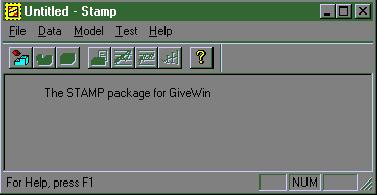
Figure 1: The main menu in STAMP 6.0
A feature of the program is the excellent range of high quality graphs that can be created to assist you in selecting a suitable model. These are much more impressive than the old *.pcx graphs that could be produced with STAMP 5.0. One of the advantages of working under Windows is that any graphs you create can be copied and pasted into other applications without the need for them to be saved separately (although graphics files can be saved in a variety of formats if you wish).
A typical session will begin in GiveWin with users loading data from a file (which can be in a variety of formats including GiveWin's own format or Excel and Lotus spreadsheet formats).(note 4) Next you might wish to use the Calculator tool to carry out preliminary transformations of the series such as differencing or taking logarithms.(note 5) You would probably also use GiveWin to create a number of graphs prior to model formulation and estimation. Figure 2 shows GiveWin in operation, with several windows open - the Results window which is where all the statistical results are sent, a window with the data file (in this case it is called Senergy) and a grapics window that shows time series plots of the series to be modelled and its first difference. The series is LTOTEe, which is the logarithm of a quarterly series of Total Final Consumption of Electrical Energy for the UK. It can be seen to have an upward trend with a pronounced but evolving seasonal pattern.
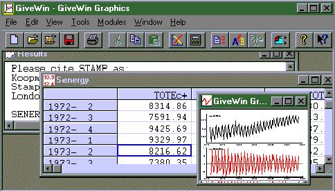
Figure 2: An illustration of the use of GiveWin with STAMP 6.0
When you are ready to formulate a model you can switch to STAMP either by clicking on the STAMP Taskbar at the bottom of the screen or by selecting an appropriate option from the drop-down GiveWin Modules menu.
Just as in recent versions of PcGive you first select the variable (or variables) that you need in the model from the right hand pane so that they appear in the left hand pane (see Figure 3). Here we will construct a simple univariate model for the series LTOTEe.
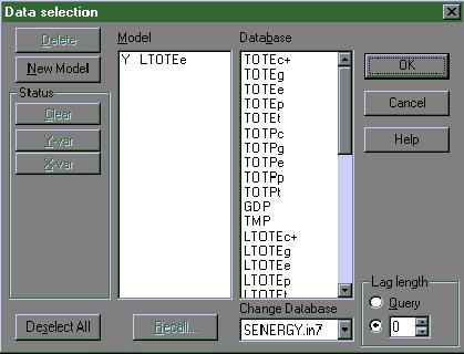
Figure 3: Model formulation in STAMP 6.0 - selecting the data series to be included in the model
Next you move on to select suitable settings for the components. Here we chose first to select a format for the trend which allows it to take its most general stochastic form with both the level and slope being permitted to evolve stochastically over time. The seasonal component is also allowed to evolve over time - the dummy setting is stochastic rather than fixed.
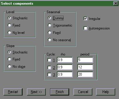
Figure 4: Selecting the stochastic component settings in STAMP 6.0
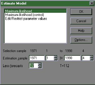
Figure 5: The model estimation dialog in STAMP 6.0
If necessary one can incorporate impulse or step dummies to allow for exceptional temporary shocks or more permanent shifts in the series prior to estimation. One can also retain some of the data series for post-sample forecasting tests (as shown in Figure 5). The initial set of results, in the form of a diagnostic summary report and estimates of the model's hyperparameters, is then sent to the Results window in PcGive (see Figure 6).
Eq  1 : Diagnostic summary report.

Estimation sample is 1971. 1 - 1995. 4. (T =  100, n =   95).
Log-Likelihood is 318.213 (-2 LogL = -636.427).
Prediction error variance is 0.00104836

Summary statistics
                  LTOTEe
 Std.Error      0.032378
 Normality        12.181
 H( 31)          0.34381
 r( 1)          0.098590
 r( 9)           0.24256
 DW               1.7720
 Q( 9, 6)         13.567
 Rs^2            0.48036


Eq  1 : Estimated variances of disturbances.

Component        LTOTEe (q-ratio)
Irr          0.00035045 ( 1.0000)
Lvl          0.00020868 ( 0.5955)
Slp             0.00000 ( 0.0000)
Sea         4.6937e-005 ( 0.1339)
|
Figure 6: Diagnostic summary report and estimated hyperparameters for our model.
Here we see that the slope hyperparameter (the variance of the disturbance term connected with the slope component) has an estimated value of zero. This suggests that the trend does not have a stochastic slope. The diagnostics are generally acceptable, although the statistic used to test for Normality (the Doornik-Hansen correction to the Bowman-Shenton statistic) suggests that there may be a problem of some sort. Moving to the Test menu we can create a graph plot and histogram of the residuals (see Figure 7). It is clear that there is an outlier in 1974 - something we should have anticipated as this was the time of the oil price shock. We can now reformulate the model to include an impulse dummy to improve both the fit and model diagnostics.
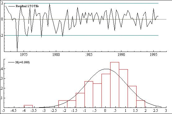
Figure 7: Selected residual graphics for our model
Figure 8 shows a more extensive set of results that have been produced for a modified model which includes an impulse dummy (intervention) for 1974Q1 but which has a fixed slope for the trend component. Further analysis of the model, including an examination of its post-sample forecasting performance (not shown here), confirms that it provides a suitable description of the series.
Equation  2.

LTOTEe = Trend + Dummy seasonal + Interv + Irregular

Estimation report
Model with  3 parameters ( 1 restrictions).
Parameter estimation sample is 1971. 1 - 1995. 4. (T =  100).
Log-likelihood kernel is 3.235707.
Very strong convergence in   6 iterations.
( likelihood cvg 9.771945e-014
  gradient cvg   4.996004e-009
  parameter cvg  6.046827e-007 )

Eq  2 : Diagnostic summary report.

Estimation sample is 1971. 1 - 1995. 4. (T =  100, n =   95).
Log-Likelihood is 323.571 (-2 LogL = -647.141).
Prediction error variance is 0.000861547

Summary statistics
                  LTOTEe
 Std.Error      0.029352
 Normality        4.2339
 H( 31)          0.49790
 r( 1)          0.074910
 r( 9)           0.15453
 DW               1.8096
 Q( 9, 7)         11.161
 Rs^2            0.57295


Eq  2 : Estimated variances of disturbances.

Component        LTOTEe (q-ratio)
Irr          0.00019649 ( 0.8749)
Lvl          0.00022458 ( 1.0000)
Sea         5.4351e-005 ( 0.2420)

Eq  2 : Estimated standard deviations of disturbances.

Component        LTOTEe (q-ratio)
Irr            0.014017 ( 0.9354)
Lvl            0.014986 ( 1.0000)
Sea           0.0073723 ( 0.4920)

Eq  2 : Estimated coefficients of final state vector.

Variable      Coefficient      R.m.s.e.       t-value
Lvl                8.7655      0.013164        665.88  [ 0.0000]
Slp             0.0042033     0.0015179        2.7691  [ 0.0068]
Sea_ 1           0.084215      0.011478         7.337  [ 0.0000]
Sea_ 2           -0.13274      0.010378        -12.79  [ 0.0000]
Sea_ 3          -0.086550      0.010286       -8.4146  [ 0.0000]

Eq  2 : Estimated coefficients of explanatory variables.

Variable      Coefficient      R.m.s.e.       t-value
Irr 1974. 1      -0.11111      0.023519       -4.7241  [ 0.0000]

Eq  2 : Seasonal analysis (at end of period).

Seasonal Chi^2( 3) test is 374.157  [0.0000].

                 Seas  1     Seas  2     Seas  3     Seas  4
 Value           0.13507   -0.086550    -0.13274    0.084215


Normality test for Residual LTOTEe
Sample Size     95
Mean                   0.031605
Std.Devn.              0.994221
Skewness              -0.412999
Excess Kurtosis       -0.284620
Minimum               -2.641913
Maximum                1.900131
Skewness  Chi^2(1)       2.7007  [0.1003]
Kurtosis  Chi^2(1)      0.32066  [0.5712]
Normal-BS Chi^2(2)       3.0213  [0.2208]
Normal-DH Chi^2(2)       4.2339  [0.1204]

Goodness-of-fit results for Residual LTOTEe
Prediction error variance (p.e.v)              0.000862
Prediction error mean deviation (m.d)          0.000696
Ratio p.e.v. / m.d in squares                  0.975170
Coefficient of determination       R2          0.973591
... based on differences           RD2         0.977656
... based on diff around seas mean RS2         0.572953
Information criterion of Akaike    AIC        -6.896781
... of Schwartz (Bayes)            BIC        -6.688367
|
STAMP 6 improves upon earlier versions of the program. Not very much has been changed in the underlying econometrics of the program in the upgrade from STAMP 5 to STAMP 6.0(note 6) . However by converting the program so that it runs under Windows the authors have produced a piece of software that looks more professional and up to date and is also simpler and more intuitive to use.
The program is very flexible in the way that it operates. Users can formulate, estimate, test and reformulate models on the basis of an extensive set of statistical and graphical output. Obviously the more familiar one is as a user with structural time series models and their properties the more effective one can be in using STAMP to arrive at a suitable model for one's purpose. However, by working through the tutorials that are built into the book using the data sets provided as files with the software, even those who are inexperienced with structural time series modelling can use STAMP to familiarise themselves with this approach.
We did find some glitches(note 7) and irritations in the performance of the program but these are relatively minor and hopefully will be attended to in various partial updates. For example, when one modifies the stochastic settings of a model (say by fixing the slope coefficient rather than allowing it to follow a stochastic process as we did as we moved from model 1 to model 2 above), any impulse dummies that may have been set up will be lost and would need to be reset. Not all of the calculated test statistics are followed by probability values or some other indicator of the level of significance of the test (such as placing an asterisk next to significant values). However the authors of the program are very responsive to feedback from users and it is expected that these features will be introduced into partial updates.
Overall, we like the new version of the program and agree with the authors when they say that it "...bridges the gap between theory and its application - providing the necessary tool to make interactive structural time series modelling available for empirical work." (Koopman et al. (2000). Preface).
STAMP 6.0 is available from Timberlake Consultants Ltd, Ujit 3, Broomsleigh Business Park, Worsley Bridge Road, London SE26 5BN, United Kingdom. Telephone +44 (0)20 86973377, Fax +44 (0)20 86973388. E-mail: info@timberlake.co.uk (or timberlake-consultancy.com in North America). Web: http://www.timberlake.co.uk/ (or http://www.timberlake-consultancy.com/ in North America).
Single user - Ł500 (Ł250 for academics, Ł85 for students); 2-5 users Ł1000 (Ł600 for academic institutions); 6-10 users Ł1500 (Ł900 for academic institutions); unlimited number of users Ł2500 (Ł1500 for academic institutions);
1 A logarithmic transformation is often first applied to a series so that these components effectively interact in a multiplicative form.
2 The CD also contains files for some other members of what is now called the OxMetrics family (econometrics modules that link up with GiveWin). However in order to install these programs from the CD a user must enter a valid licensing code.
3 You can also download a free demo version of STAMP from the web site http://www.ssfpack.com/stamp [Now at http://stamp-software.com/- Web Editor]. This is the place to get the very latest news about the program.
4 GAUSS and STATA files are also amongst the list of supported formats.
5 You can use the Algebra editor if you wish to program more complex transformations or to call up a set of instructions that has been used previously and saved to disk.
6 The normality test has been updated to give the Doornik-Hansen correction to the Bowman-Shenton statistic. Some other changes have been made that affect the way the results are presented. For example the estimated hyperparameters are now provided directly (as variances of the disturbances) as well as in standard deviation form. The labels on seasonal components when they are graphed have been changed so that Seas 1 always refers to the first season of the year, rather than being used for the first seasonal of the estimation period.The default settings for the convergence of the numerical optimisation process have been slightly increased which may affect the results slightly if one makes a comparison with those obtained using STAMP 5.0.
7 Several programming bugs that were present in the original release of STAMP 6.0 have now been fixed. Check the program's web site for the latest list of bugs and for updates to download.
Doornik, J. A. and D. F. Hendry (1999) GiveWin: An Interface to Empirical Modelling. Timberlake Consultants.
Harvey, A. C. (1989) Forecasting, Structural Time Series Models and the Kalman Filter. Cambridge: Cambridge University Press.
Harvey, A. C., S. G. B. Henry, S. Peters and S. Wren-Lewis (1986) "Stochastic Trends in Dynamic Regression Models: An Application to the Employment-Output Equation." The Economic Journal, Vol. 96 (December) pp 975-985.
Harvey, A. C and A. Scott (1994) "Seasonality in Dynamic Regression Models." The Economic Journal, Vol. 104 (November) pp 1324-1345.
Harvey, A. C. and N. Shephard (1993) 'Structural Time Series Models'. In Handbook of Statistics, Vol. 11 (ed. G. S. Maddala et al.). Barking: Elsevier Science Publishers.
Judge, G. (1995) "STAMP 5.0" Computers in Higher Education Economics Review Vol 9 Issue 3 pp 28-30.
Judge, G. and Y. Ninomiya (2000) "STAMP 6.0" The Economic Journal. Vol 110 No 467 (November) pp F720-F738
Koopman, S. J., A. C. Harvey, J. A. Doornik and N. Shephard (2000) STAMP: Structural Time Series Analyser Modeller and Predictor. Timberlake Consultants.
Scott, P. and G. Judge (2000) "Cycles and steps in British commercial property values." Applied Economics Vol 32 No 10 pp1287-1297.