Volume 11, Issue 1, 1997

Economic Optimisation using Excel's Solver
- a macroeconomic application and some comments regarding its limitations.
- John Houston
- Glasgow Caledonian University
Introduction
Recent issues of this review have included papers regarding economic optimisation. Two of these (
MacDonald 1995,
1996) have extolled the virtues of Excel's Solver as a user-friendly and flexible tool for economic optimisation. Both these papers have described the application of the Solver to simple Linear (and Integer) Programs as used by that author in his teaching, and stress the ease with which students can set up and solve models of this nature. The purpose of this paper is twofold : firstly to describe another economic application of the Solver as used in the author's teaching and research and secondly, to make some general comments on the limitations of the Solver as an modelling tool.
Intertemporal Optimisation
Another advantage from using Excel's Solver (as opposed to LINDO, for example), is that it makes it possible to construct and solve optimisation models that have an
intertemporal dimension to them. Many problems in Economics require an optimal set
of decisions, with one to be made in each of several time periods. Optimal in this sense implies that the modeller wishes to maximise (or minimise) some
total amount over the entire period covered by the model. The important distinction to be made between this and 'one-off' optimisation is that any single decision may not be optimal in itself, but that it is one part of a grander plan to optimise over the longer run. So, for example, we might expect a very short-lived agent to consume all of his wealth in the single period of his life - this is optimal. However, a longer lived agent must eke out his wealth over his lifetime, implying that he cannot consider consuming it all in one period. Any decision to do so will most certainly not be inter-temporally optimal.
Macroeconomic theory has been preoccupied with trying to understand the relationship between aggregate consumption and aggregate income. Researchers working in this area assume the existence of a rational, representative economic agent who wishes to maximise his total lifetime utility from consumption. Each period, the agent has to make a decision regarding how much of his wealth he should spend on goods and services and how much of current income should be saved or how much he should borrow. The author has taught elements of this theory on second- and third-level courses in economic modelling and macroeconomics, and has found the Solver to be an invaluable tool in bringing life to the concepts explained in the lectures. Students construct models similar to the one that will be described in this paper, then use the Solver to determine the agent's optimal period-by-period consumption. They can then alter the models' parameters and observe the impact of these changes on the pattern of consumption. Thus, for example, they can better appreciate the influence of the initial endowment and the rate of interest on the accumulation of wealth and the consumption pattern; the rate of discount applied to utility in increasing the agent's 'impatience' to consume
earlier and; the importance of the assumptions made about the form of the agent's utility function.
The basic model
The model described here will be the simplest of the family used by the
author. A considerably more complex model is described in
Houston and Gasteen (1997), which,
inter alia,
generates aggregate consumption functions from ind ividual intertemporal
functions and demographic profiles for the UK economy. The model
described here starts by making the following assumptions :
- Utility is derived only from current consumption. The utility
function is assumed to belong to the logistic class, and is given
as
 , where a and b are parameters and
ct is consumption in
period t. This is only one of several competing forms, but has
the attraction of modelling diminishing marginal utility. Whilst the
student cannot change the general form of the utility function, it
is possible to alter its parameters.
, where a and b are parameters and
ct is consumption in
period t. This is only one of several competing forms, but has
the attraction of modelling diminishing marginal utility. Whilst the
student cannot change the general form of the utility function, it
is possible to alter its parameters.
- It is assumed that utility has no 'time value' i.e. the present value of one 'util' this year is worth exactly as much as one to be realised in 50 years time. The student can however, model and observe the effect of time-discounting utility and its tendency to encourage consumption sooner, rather than later in life.
- The agent is given an endowment at the start of his life which is immediately available for consumption. It is also assumed that he will die with nothing, though, again, students can require him to bequeath some capital upon death.
- The agent's only income is interest from his accumulated wealth
(measured at the start of each period). He may decide to consume only
part of his current income, adding the rest to wealth for subsequent
reinvestment and income generation. On the other hand, he may consume
more in a period than he has income, thereby reducing his wealth (and
future capacity to generate income, given the assumed real rate of
interest). A single rate of interest is assumed to apply throughout the
agent's life, though different rates can be incorporated if required. It
is also assumed that the rate of interest on income and the rate of
discount on utility are independent. It would be fairly simple to link
the two by modelling the discount rate as a function of the interest rate,
or both as a function of wealth.
- Consumption is constrained from above by the total wealth available
and obviously, from below, by zero. In the interests of realism, the
student can specify a minimum 'starvation' level of consumption per
period, lest the Solver find it optimal to set consumption to very low
levels in some periods.
The basic spreadsheet model is
illustrated in Figure 1, with the logic for the first period displayed in
full. This can then be copied across the columns for as many periods as
the agent is assumed to live (with the proviso that from the second period
on, the wealth brought forward is last period's wealth carried forward).
This particular model assumes a 50-period lived agent, with no
non-negative lower bound on consumption, who inherits �1000, with wealth
attracting 10% interest per period. The logic is very simple, and can be
quickly constructed and interpreted by the average undergraduate. In
addition, it is very simple to alter any of the parameters of the model
and observe the effect on consumption. Notice that row 15 (apart from
A15) is left blank at this stage. It is into these cells that the Solver
will trial various consumption levels in its effort to maximise this
agent's utility given the constraints imposed on the model.
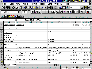
Figure 1 Structure and Logic of the Spreadsheet Model
Setting up the Solver
Instruction in how to set up the Solver is given in both of MacDonald's
papers and need not be repeated here. Figure 2 illustrates how the Solver
Dialogue Box should look like for this model. Obviously, we wish to
maximise total utility (
E1) by allowing consumption to change
(
B15 outwards). The first constraint ensures that the agent leaves
at least a minimum amount of wealth upon his death. The second (actually
several constraints modelled jointly) ensures that the agent does not
consume more than his wealth (plus current income) in any period. This
constraint is written in such a way that each cell on both sides will be
paired together correctly (i.e.

, etc.) and saves a
lot of typing!
The third and final constraint ensures that the agent
consumes at least some minimum amount in each period (a 'starvation'
level), as specified in B4.
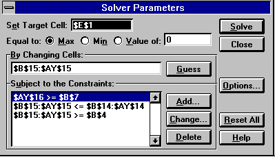
Figure 2 The Solver Dialogue Box
Solving the Model
Once this has been set up, the student then clicks on the Solve button and
awaits the result. When Solver has found an optimal solution (after about
100 iterations taking 5 minutes), the consumption row (
# 15) will
have a series of amounts which have been placed there by the Solver. It
is from these that period utilities are calculated and summed in
E1. This is the maximum utility this agent can obtain in his
lifetime given the parameters. From this, the student can produce graphs
of consumption, income and wealth over time (Figure 3) as well as
consumption versus income (Figure 4).
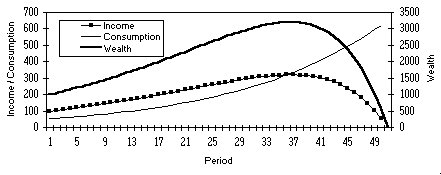
Figure 3 Consumption, Income & wealth over the agent's lifetime
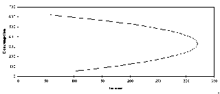
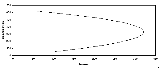
Figure 4 Intertemporal Consumption Function for the representative agent
Altering the assumptions
Having solved the model, the student can then make changes to any of its parameters. Whilst various combinations of changes can be tried, it is probably better from a pedagogic viewpoint to examine the effects of altering just one parameter at a time.
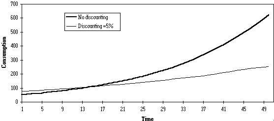
For example, the student may be interested in learning what effect time-discounting utility has on the lifetime pattern of consumption. This can be done by first using
Copy - Paste Special - Values to store the consumption figures from the original, undiscounted model to another part of the sheet, increasing the discount rate (in cell
B9), then resolving the model. The new consumption levels can be pasted to a row or column adjacent to the originals, and both plotted against time (Figure 5).
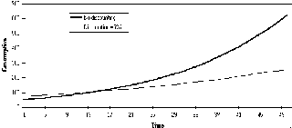
Figure 5 Consumption profiles for 0% and 5% discounting
In this case, student can see that reducing the real value of future utility (in relation to the rate of interest) makes the agent more impatient to consume in the early stages of his life. As a result, he retains less of his wealth in the early stages, which lowers the amount of Capital on which later Income can be earned. As a result, the agent cannot consume at the same level in later life.
Problems will occur where the student unwittingly generates a scenario for which there is no feasible solution. For example, it is obviously impossible to insist on a minimum level of consumption (per period) that would result in all wealth being
consumed long before the end of the agent's life. In this example, the agent has an endowment of �1000 and a 10% return on wealth to last him say, 50 years. Roughly speaking therefore, average annual income will be �100. If the starvation level of consumption is set above �100, then no feasible solution can exist, given the assumptions of the model. This would be complicated further by insisting that some wealth be bequeathed upon death - the greater the bequest, the tighter will be the rein on consumption, and the greater the chance of there being no solution. There is no way of prechecking the feasibility of the problem as set before attempting to solve it (except where it is obvious), thus there is always the risk of waiting for a solution that never comes. The student will be informed if the Solver can't find a solution, in which case the student needs to go back to the model and look to relax some of the constraints.
The ease with which models can be set up and solved clearly makes the Solver a useful tool in teaching and research. That said, this author has experienced some of its shortcomings which presently limit its application to relatively small, simple models, such as the one described above. Two limitations in particular are worth mentioning, viz.,
- Time taken to solve larger models.
- Getting trapped at a local optimum.
Time taken to solve larger models
Given the flexibility and ease of use of the Solver, the temptation always
exists to develop larger and more sophisticated optimisation models. As
well as the second- and third level classes in economic modelling, the
author teaches part of a fourth level class in business modelling. The
basis of the practical computing sessions is a spreadsheet-based cash flow
model of a single-product company. Period demands are estimated from a
set of variables, including Own Price, Competitors Price and Interest
Rate. The students then decide on the numbers of workers and machines to
employ in each period (a Cobb-Douglas technology is assumed), which can be
more or less than the demand in that period (thus permitting Stocks or
Lost Sales to occur). Factor productivities can be selected with unit
costs being drawn from lookup tables. Once the students had had time to
'manually' optimise the model by trial and error, the intention was then
to let the Solver optimise the total net cash flow over 10 periods. In
doing this, it was to be permitted to select the numbers of full- and
part-time workers, the number of machines, their rate of output and unit
prices for the finished product. The students would then compare their
best attempts with a truly optimal production plan. Unfortunately, the
time taken by the Solver to perform this task was so long, as to preclude
using it 'as live' in the practicals. Even when using a 100Mhz Pentium
PC, obtaining a solution took the best part of five hours. As most of the
teaching machines at Glasgow Caledonian are still 486 standard, the only
option was to provide students with a ready-solved model, depriving them
of the experience of setting it up and solving it. As a consequence of
this, it was not possible, for them to gauge the effect on total net cash
flow of parameter changes, such as raising or lowering unit prices.
Obviously, as the power of the teaching-lab PCs increases, then this will
become less of a problem, though it currently has to be seen as a severe
limitation on work of this kind.
Getting trapped at a local
optimum
An ever-present problem of any 'hill-climbing' optimisation technique, is
that it can arrive at what appears to be the optimum solution, when in
fact it is only a local one. Solver trials solutions and moves in the
direction that appears to yield the fastest rate of change in the value of
the objective function. Once it gets to a point where there appears to be
no further gains to be had, it stops and reports that it has found
an optimum solution. The temptation is always to take this as
the optimum solution. However, the author has experienced several
cases where running the Solver from different 'starting' locations has
resulted in different optimum solutions being obtained. This happens, for
example, when the objective function's surface is comprised of 'spikes'
(see Figure 6), as a result of the complexity of the underlying
relationship between the objective and the causal variables.
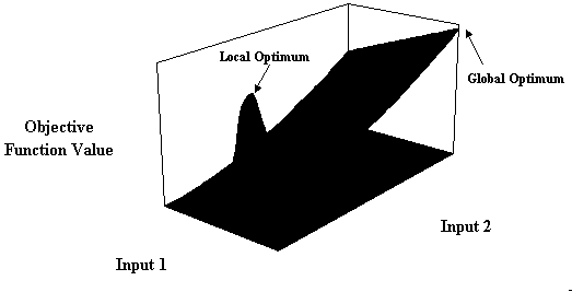
Figure 6 Objective Function Surface with local and global optima
As can be seen from this rather exaggerated example, should the search
start with a low value for Input 1, then there is a good chance
that it will be drawn to the local peak. On the other hand, if the model
was seeded to start from a higher Input 1 value, then there would
be a much better chance of finding the true global optimum. Of course, it
is only possible to plot the objective function surface for a model with
one or two inputs, thus the only practical solution is to run the model
several times using different seed values. In the event that most, if not
all, of the runs yield the same solution, you can be reasonably sure that
you have the true optimum.
References
- Houston, J. and Gasteen, A., 1997
- "From the general to the specific : estimating aggregate intertemporal consumption functions from survey data", Department of Economics Discussion Paper, Glasgow Caledonian University.
- MacDonald, Z., 1995
- "Teaching Linear Programming using Microsoft Excel Solver", Computers in Higher Education Economics Review, 9 (3), 7-10
- MacDonald, Z., 1996
- "Economic optimisation : an Excel alternative to Estelle et.al's. GAMS approach", Computers in Higher Education Economics Review, 10 (3), 2-5
Address for correspondence:
John Houston, Department of Economics, Glasgow Caledonian University, Cowcaddens Road, Glasgow, Scotland, G4 0BA
E-mail
J.Houston@gcal.ac.uk