Volume 17, 2005
Incorporating Explanatory Variables into Risk Simulation Models
- Michael Backus
- Service Manager, Wells Fargo Glennallen
Abstract
A handful of articles have already been written describing how Excel can be used to model financial uncertainty via Monte Carlo simulation. Unfortunately, to date the methods described have been useful only for education purposes. This article describes how to incorporate explanatory variables into one’s models, giving Excel users the ability to model complex scenarios on a level comparable to programs designed specifically for simulation purposes such as @Risk and Crystal Ball. And best of all, it is extremely educational and a practical real world skill.
Introduction
Risk simulation being a topic of fundamental importance to the economist, investor and entrepreneur, it is regrettable that more universities and economics textbooks do not adequately cover its mechanics. Luckily, two CHEER papers have been written concerning this topic (Judge, 1999; Smith, 2000). Unfortunately, neither demonstrated how to model explanatory variables. What follows is an explanation of how to incorporate explanatory variables into the Excel-based risk simulation models outlined by Smith (2000).
Before continuing, I would first like to explain why learning this technique is worthwhile when programs like Crystal Ball and @Risk are available.
- For many, Excel is the only readily available program capable of carrying out such powerful analysis. While there are Excel add-ins that may be purchased specifically for this purpose, to most they are prohibitively expensive – the basic versions of @Risk and Crystal Ball cost approximately $770 and $685 respectively! (Imagine the cost of equipping an entire computer lab.)
- Excel is a standard program found on most computers. One may email a model to peers, who can then provide valuable feedback. If the model is created for release to the general public, almost anyone will be able to use and audit it.
- Excel provides the ideal learning atmosphere. Its extensive set of basic capabilities allows students to tackle almost any project. Yet, to accomplish tasks such as Monte Carlo simulation, students must understand exactly what they are doing. (There is no ‘black box’ into which inputs are dumped and from which results are received.)
Correct specification of parameters
Before delving into the mathematics behind risk simulation, I would like to issue the following warning. In essence, Monte Carlo simulation is nothing more than running regression backwards. Instead of estimating parameters given a set of data, one simulates data using parameter estimates. However, there are some important differences. While most students of statistics understand that departures from ordinary least squares (OLS) regression such as non-constant or non-normal errors can be a nuisance, few realise the magnitude that such problems present when using coefficients estimated in such a manner. This is because many statistical studies focus on the means of slope coefficients, asking such questions as ‘Does group A differ significantly from group B?’, ‘Does a change in X significantly impact Y?’ and ‘Given the explanatory variables, what is the best guess at the next Y to be observed?’ When asking such questions, the statistician may rightfully gloss over the aforementioned departures, as OLS is somewhat robust (or resistant) to their effects. That is, relatively minor cases of non-constant variance or non-normal errors will not generally impede one from detecting significant slopes or significant differences between groups, or from making accurate guesses at the next value. However, simulating data is to ask an entirely different question: ‘What are likely values for the next Y to be observed?’ Such a question entails accurate prediction intervals, which in turn entail the need for accurate estimates of the standard error of the regression, and standard errors for the coefficients.
The statistical equation must also describe the data accurately. Overly variable input will not only yield overly variable (and consequently less useful) output, but may also lead to biased conclusions. Referring back to the x2 example listed above, suppose that while the true standard deviation is 1, it is incorrectly estimated as 2. The mean output would then be 8, not 5.
Unfortunately, there is no test to determine whether statistical parameters have indeed been estimated correctly. The best course of action is to rely on theory when possible. For example, by using an exponential equation instead of a long polynomial equation to model inflation, future estimates will almost certainly be more accurate. Also, it is always a good idea to compare many simulations to the original data. By doing this, one can quickly see whether trends and/or variation behave similarly to the original data.
Mathematics behind Monte Carlo simulation
Of course, the first tool necessary for simulating data is a correctly specified model. Most statistical packages will provide most of the necessary data – coefficient estimates and the standard error of the regression. With these, one can accurately simulate variation about a trend line. However, it must also be remembered that, since trend lines are estimated from samples, they are also subject to error. Unfortunately, one cannot simply use the standard errors of the coefficients to simulate trend lines. This is because a trend line’s coefficients are correlated.
To account for the variation of the trend line, it is necessary first to calculate the variance covariance matrix of the coefficients, as shown below.
σ2{b} = σ2(X' X)–1
Once this has been done, it is necessary to calculate the square root of the variance covariance matrix (to obtain something analogous to the ‘standard deviation matrix’). This gives rise to a peculiar situation, as there can be many square roots to a single matrix. Luckily, any matrix S that satisfies the following condition can be termed the square root of matrix M, and used to create simulated trend lines.
SS' = M
Using explanatory variables to simulate risk in Excel
Although Excel is not sold with the capability of carrying out this calculation, the University of Chicago distributes a freeware Excel add-in called Simtools that can be downloaded at http://www.kellogg.nwu.edu/faculty/myerson/ftp/addins.htm . Simtools augments Excel’s abilities with 32 additional statistical functions.(note 1) One of these new functions, ‘MSQRT’, calculates the Cholesky factor, which is a lower triangular matrix (all elements in the upper right portion are zero) that has the following properties:
C'C = M but CC’' ≠ M
When simulating data, it is important that, however defined, the left-hand matrix is used.
Once all parameters have been calculated, one can begin building the simulation. To simulate a trend line, a matrix of standard normally distributed random errors must be created that has as many rows as parameters (but only a single column). This is easily accomplished in Excel by using the ‘RAND()’ function in conjunction with the ‘NORMINV’ function. Simply type the following in each cell:
“=NORMINV(RAND(),0,1)”
The last two arguments indicate a mean of zero and a standard deviation of 1. Multiply the transposed Cholesky factor by this matrix of standard normally distributed random numbers to create deviations from the parameter estimates. Then simply add these deviations to the parameter estimates to create simulated parameters.
![[Cholesky Factor][Random Numbers] + [Parameter Estimates] = [Simulated Parameters]](backus1.gif)
When these are multiplied by their respective explanatory variables, the result will be a simulated trend line. To simulate variation about the trend line, all one must do is add a random error to each observation. This can be done by typing:
“=NORMINV(RAND(),0,SQRT(MSE))”
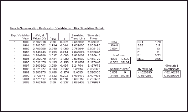
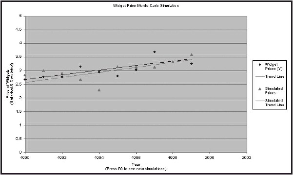
where “SQRT(MSE)” denotes the standard error of the regression. For a simple working example of how to do this in Excel, please see the Widget Price Monte Carlo Simulation.
Applications
Once data have been simulated, it is a simple matter to plug these values into any risk simulation model similar to that outlined by Smith (2000). Note that this method not only works for normal data, but also can be applied to any non-normal data that can be transformed so that they are normal (such as log-normal data). Furthermore, it is possible to model complicated explanatory variables like auto-regressive and moving average components so long as the parameters are estimated using more advance programs like SAS.
Conclusions
By using this technique, it is possible to mirror real-world phenomena much more accurately. Hence, understanding this technique allows one to ‘bridge the gap’ and use Excel on a par with more expensive programs such as Crystal Ball and @Risk. In fact, learning this method may prove a valuable skill to recent economics graduates wishing to conduct complicated real-world risk analysis. At the very least, it will result in a much better understanding of what goes on in Crystal Ball’s and @Risk’s ‘black box’.


Contact details
Michael Backus
Service Manager Wells Fargo Glennallen
Wasilla, Alaska
USA
Tel: (907) 822-3214
Email: mbackus_alaska@yahoo.com
Notes
1. Roger Myerson teaches a class at the University of Chicago, and has posted many homework assignments (accompanied by answers) which utilise the features of the Simtools add-in at http://home.uchicago.edu/~rmyerson/econ205.htm .
References
Judge, G. (1999) ‘Simple Monte Carlo studies on a spreadsheet’, Computers in Higher Education Economics Review, 13(2), pp. 12–14.
Smith, D. J. (2000) ‘Risk simulation and the appraisal of investment projects’, Computers in Higher Education Economics Review, 14(1), pp. 9–13.

