Volume 14, Issue 2, 2000
Review of EViews 4.0
- Paul Turner
- Department of Economics, University of Sheffield
Introduction
EViews 4.0, the new version of the popular econometrics package, became available in January 2001. Existing users of the package will find the interface familiar but improved in terms of the presentation of graphics and increased flexibility in terms of data handling. For many simple applications, users will probably not notice any major changes in the new version. However, there have been significant changes in a number of areas which I discuss in this review.
Modelling
The modelling interface is probably the area in which EViews has changed most radically. In previous versions a model consisted mainly of a block of text containing a mixture of equations and comments. The new version allows several different ways of 'viewing' the model other than in text form. For example, the equation view enables the user to assess the structure of the model. This is illustrated in Figure 1, which shows the equation view for a simple income-expenditure model of the US economy consisting of a consumption function, an import demand function, the national income accounting identity and a definitional relationship for disposable income.
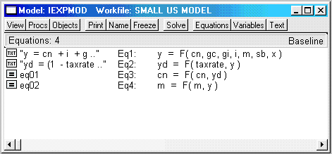
Figure 1. Equation view of a simple income-expenditure model
Alternatively, we can use the variable view shown in Figure 2 to examine the status of each variable in the model. This provides a handy way of quickly assessing which variables are endogenous and which are exogenous.
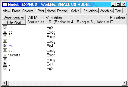
Figure 2. Variable view of the income expenditure model
There is also the standard text view of the model as well as a block structure view, which is most useful for large models that can be divided up into recursive blocks.
Once the model has been set up, version 4.0 allows the user to examine various scenarios in which the model is conditioned on alternative sets of values of the exogenous variables. This procedure takes some getting used to and requires careful reading of either the manual or the online help. However, once the user is familiar with the method, it provides a convenient way of carrying out and storing a variety of different scenarios of interest. After the model simulations have been conducted, it is possible to present the results either in table or graphical form. For example, in Figure 3, I illustrate a dynamic model simulation for GDP using a base set of data and an alternative scenario in which government consumption is increased by 5% relative to base.
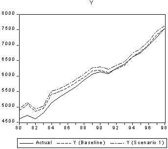
Figure 3. Dynamic simulation of the income-expenditure model under alternative scenarios
There are also new, advanced options for solving the model relative to earlier versions of EViews. For example, version 4.0 offers the alternative Newton algorithm to the standard Gauss-Seidel solution method. However, the two major innovations relative to earlier versions are: (i) version 4.0 now allows solution of models with forward-looking expectations by means of a variant of the Fair-Taylor algorithm and (ii) version 4.0 now allows automatic stochastic simulations to be carried out conditional on the standard deviations of equation objects included in the model.
Vector autoregression analysis
The output for vector autoregressions has now been considerably enhanced relative to earlier versions. In particular, version 4.0 now permits automatic calculation of pairwise Granger causality tests, presentation of residual correlograms and lag exclusion tests. For unrestricted VAR's version 4.0 also allows the calculation of a range of lag length criterion tests with an automatic indication of the lag length chosen by each. For example, Table 1 shows the lag length tests for a VAR relating the quarterly growth rates of UK consumption expenditures and disposable income.
Table 1. Lag length criteria for an unrestricted VAR
VAR Lag Order Selection Criteria
Endogenous variables: DLOG(CONS) DLOG(RPDI)
Exogenous variables: C Q1 Q2 Q3
Date: 02/27/01 Time: 10:25
Included observations: 156
Sample: 1955:1 1997:1
| Lag | LogL | LR | FPE | AIC | SC | HQ |
|---|---|---|---|---|---|---|
| 0 | 786.2011 | NA | 1.59E-07 | -9.976937 | -9.820534 | -9.913413 |
| 1 | 808.6143 | 43.10228 | 1.26E-07 | -10.21300 | -9.978399 | -10.11772 |
| 2 | 824.7080 | 30.53689 | 1.08E-07 | -10.36805 | -10.05525 | -10.24100 |
| 3 | 849.9537 | 47.25466 | 8.21E-08 | -10.64043 | -10.24942 | -10.48162 |
| 4 | 864.1974 | 26.29608 | 7.20E-08 | -10.77176 | -10.30255 | -10.58119 |
| 5 | 878.6568 | 26.32351 | 6.30E-08 | -10.90586 | -10.35845* | -10.68352* |
| 6 | 880.1814 | 2.736536 | 6.50E-08 | -10.87412 | -10.24851 | -10.62002 |
| 7 | 884.7036 | 8.000770 | 6.46E-08 | -10.88082 | -10.17700 | -10.59496 |
| 8 | 890.3664 | 9.873530 | 6.33E-08 | -10.90213 | -10.12012 | -10.58451 |
| 9 | 895.4619 | 8.753892 | 6.25E-08 | -10.91618 | -10.05596 | -10.56680 |
| 10 | 901.8756 | 10.85387* | 6.07E-08* | -10.94712* | -10.00871 | -10.56598 |
| 11 | 904.0344 | 3.597993 | 6.22E-08 | -10.92352 | -9.906899 | -10.51061 |
| 12 | 904.7681 | 1.204063 | 6.50E-08 | -10.88164 | -9.786822 | -10.43697 |
LR: sequential modified LR test statistic (each test at 5% level)
FPE: final prediction error
AIC: Akaike information criterion
SC: Schwarz information criterion
HQ: Hannan-Quinn information criterion
One of the most interesting features of the revised VAR output is the facility to examine the inverse roots of the autoregressive polynomial of the VAR. This acts as an additional check on the stability of the estimated model and gives some intuition as to its likely dynamic behaviour in terms of the decay rate of innovations and possible cyclical adjustment. These roots can be represented either in table form or as points in the unit circle, as illustrated by Figure 4.
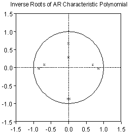
Figure 4. Inverse roots of the characteristic polynomial of a VAR
Finally, there is now the facility to allow for alternative identifying restrictions other than the standard causal ordering or Cholesky factorisation. These include structural factorisations consisting of either short-run restrictions on the interrelationships of the variables or long-run restrictions on the response of model variables to particular innovations. These require considerable care to set up properly, but are an important addition to the range of options offered in VAR analysis.
State-space estimation
State-space estimation offers an extremely flexible framework which encompasses traditional econometric estimation techniques as well as a wide variety of time-varying parameter models. EViews has had the facility to set up state-space models in previous versions, but both the interface and the range of options available have been considerably enhanced in version 4.0. A state-space object typically consists of one or more signal equations that relate observable variables to possibly unobservable state variables and a set of state equations that describe the behaviour of the state variables through time. Estimation is through the Kalman filter algorithm. This permits a very wide range of model structures, including conventional ordinary least squares, recursive least squares and time-varying parameter models.
As an example of the state-space method we have set up a version of the capital asset pricing model in which we allow the response coefficient of the daily return on Vodafone shares to the market return to follow a random walk. The estimation period is October 1995 to December 2000. The state-space object set up to estimate this model is shown in Figure 5.
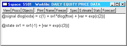
Figure 5. State-space object to estimate model with random walk coefficient
When the model has been estimated by means of the Kalman filter, we can examine the behaviour of the response to the market return by means of either the filtered or the smoothed parameter estimates. The smoothed estimates eliminate some of the variation in the series to give a clearer view of significant changes in the estimate, as shown in Figure 6. This procedure is valuable when we suspect structural change during the estimation period but are unsure as to when breaks might occur. In this case it is clear that there is a distinct increase in the responsiveness of returns on this share to market returns in the latter part of the sample.
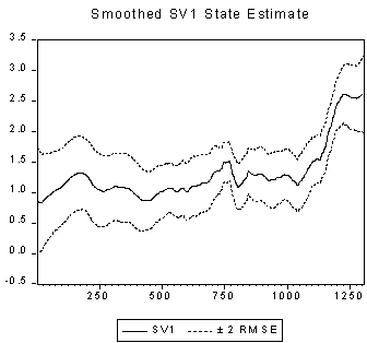
Figure 6. Time-varying estimates of the response of Vodafone returns to market returns
Summary
Users of previous versions of EViews will find the basic operations very little changed in this latest version. However, there are some important modifications to the more advanced features, such as the modelling, vector autoregression and state-space procedures. I found that the new modelling procedures were initially rather awkward to use. In some cases I had already written programes to carry out these procedures (forward-looking expectations, stochastic simulation, etc) and found the built-in procedures less flexible, although it has to be said they would be much easier for a newcomer to the package.
The vector autoregression procedures mark a considerable improvement on earlier versions in terms of both the ease of use and the quality of the output. The automated lag length criteria and the inverse roots of the autoregressive lag polynomial are particularly welcome additions. State-space estimation procedures have also been significantly improved.
In summary, EViews 4.0 has improved considerably on earlier versions by the addition of new features. The interface has changed only slightly, but users of more advanced features will quickly become aware of the increased power of the latest version in carrying out state-of-the-art econometric analysis.
Contact details
Dr P.M. TurnerDepartment of Economics
University of Sheffield
9 Mappin Street
Sheffield S1 4DT
United Kingdom Tel: 44 (0)114 2223404
Fax: 44 (0)114 2223458
Email: p.turner@sheffield.ac.uk
For further details about EViews, see its entry in the Economics LTSN Software Catalogue.

