

In a recent paper Judge (1999) explored the scope for using a spreadsheet to carry out Monte Carlo studies. The rationale was the availability of inexpensive computing power combined with the facilities made available on a spreadsheet like Excel.
This paper follows a similar vein examining one type of application that relies upon Monte Carlo experiments. Risk simulation relies upon Monte Carlo experiments to model the uncertainty surrounding decisions. It is often used in association with investment appraisal. As such it falls within the domain of Managerial Economics. The teaching of investment appraisal on managerial economics modules has been transformed by the widespread availability of spreadsheets. With a spreadsheet one can demonstrate the concepts of discounting and the time value of money (Bridge, 1989). More significantly spreadsheets make it possible for students to work independently exploring these concepts for themselves. Students can now construct an investment appraisal model and conduct a 'what if' analysis to explore the consequences of changes in the parameters of the model such as income projections and interest rates.
Risk simulation forms an important part of investment appraisal, not least because it offers a means of examining the impact of uncertainty. Nor is this necessarily confined to managerial economics, many leading texts on strategic management (Johnson and Scholes, 1999) incorporate risk analysis into the evaluation of new or different strategies.
While investment appraisal can easily be conducted using a spreadsheet, risk simulation is more problematic. Risk simulation models are more sophisticated than investment appraisal models. They involve the use of Monte Carlo experiments, which if they are to produce meaningful results have to be undertaken a large number of times. This requires some form of control structure in order to 'automate' and speed up the experimentation process. Because of this, a number of specialist 'add-in' packages have been developed, such as '@Risk' and 'Crystal Ball'. These make risk simulation with a spreadsheet straightforward. A number of articles and texts (Jones and Sheard, 1991; Oakshott, 1997; Vose 1996; Uyeno, 1992; Barlow, 1999) have described the risk simulation applications using @Risk. Unfortunately such packages are not always widely available and students may not have access to them.
While it is possible to undertake risk simulation on a spreadsheet without using a specialist add-in package (Bodily, 1986), to complete a large number of Monte Carlo experiments is slow and time consuming. The macro programming facilities available with more advanced spreadsheets mean that it is possible to set up a risk simulation model that will conduct a large number of experiments or simulations on a non-manual basis. A number of papers (Smith, 1994; Seila and Banks, 1990; Diacogiannis, 1994) have shown how simple models of this type can be developed. The advent of later versions of Excel with facilities for programming in Visual Basic for Applications (VBA) takes the process a stage further and allows the creation of complex control structures that permit the development of sophisticated models.
The purpose of this paper is to show how such models can be developed. The paper also takes the opportunity to explore some of the uses to which students can put risk simulation models in order to make themselves thoroughly conversant with the technique. Hopefully this forms a useful supplement to Judge's (1999) recent paper on Monte Carlo studies.
Risk simulation is a risk analysis technique that came to prominence in the early 1960s (Hertz, 1964). It involves the use of a probability distribution and random numbers, hence the Monte Carlo element, to estimate net cashflow figures. When discounted these figures sum to an estimated net present value (NPV) for a project. Repeated many times one gets a distribution of project NPV. If the resulting distribution is presented as a graph it is relatively easy to comprehend the uncertainty surrounding a project. This is beneficial for students because it contrasts sharply with the deterministic nature of most investment models.
The construction and operation of a risk simulation model for an investment appraisal application involves a number of steps.
| Step 1: | Build an investment appraisal model using discounted cashflow. | |||
|---|---|---|---|---|
| Step 2: | For each year's net cashflow create a probability distribution and link it to a random number generator. | |||
| Step 3: | Carry out a simulation by drawing a value from each probability distribution using the random number generator and sum the resulting estimates to provide an overall estimate for project NPV. | |||
| Step 4: | Repeat the simulation many times (i.e. 500 or more) to provide an estimated distribution for NPV for the project. | |||
| Step 5: | Decide whether the probability that the project NPV may be negative is, or is not an acceptable risk and proceed accordingly. | |||
| Year | Discount Factor | Net Cashflow | Present value |
|---|---|---|---|
| 0 | 1 | -85000 | -85000 |
| 1 | 0.9091 | 25000 | 22727 |
| 2 | 0.8264 | 25000 | 20661 |
| 3 | 0.7513 | 25000 | 18783 |
| 4 | 0.6830 | 25000 | 17075 |
| 5 | 0.6209 | 25000 | 15523 |
| NPV | 9770 | ||
Table 1: Simple Model
Table 1 shows a simple DCF investment appraisal model that can form the basis of a risk simulation. It utilises cells B2:E11 on the spreadsheet. It is an entirely conventional DCF model. In column one are the years that the project is operational (B4:B9). The third column shows the estimates of net cashflow for each year together with the initial cost of the project (D4:D9). In this instance the initial cost of the project (i.e. purchase of machinery) is Ł85,000 and the net cashflow is Ł25,000 each year for five years. In the second column (C4:C9) is the discounting factor. For year 0 the value of the discounting factor is one, because it represents the present time. Thereafter the discounting factor is based on the formula:
PV = 1/(1 = r) n
where PV is present value, r is the discount rate and n is the year. In this instance a discount rate of 10% is used and the project has a life of 10 years. The discount rate is located in cell C28. This forms part of the Summary section located in cells B27:E32. Implementing the discounting formula for cell C5 gives the formula:
+1/(1 + $C$28)^B5
This formula can be copied into cells C6:C9. Column four (E4:E9) shows the present value of the cashflows, being the result of applying the relevant discount factor to the relevant net cashflow. In cell E11 is the overall NPV for the project represented by the formula:
+Sum(E4:E9).
In order to implement a risk simulation the following additional capabilities are required of a spreadsheet:
All of these capabilities are to be found in most modern spreadsheets, but Excel has the advantage that Visual Basic for Applications provides greater flexibility in creating sub-routines.
To undertake Step 2 the estimated cashflow figures in column two of Table 1 are replaced by a random variate sampled from an appropriate distribution that represents the range and frequency of likely values for this entity. In this instance a normal distribution is used. New values will be generated every time the spreadsheet is recalculated. The probability distribution is represented by a mean value and associated standard deviation. To be consistent with the simple model a mean of Ł25,000 is used and a standard deviation of Ł10,000. Identical values are used for every one of the five years of the project. It is the standard deviation that reflects the level of uncertainty. A high value for the standard deviation, as in this case, means a high level of uncertainty and thus a high level of risk. One would expect this to be reflected in the resulting distribution for project NPV.
The probability distribution and random number generator are combined by using the formula: a + b* (RAND() + RAND()...RAND() - 6) where a is the mean (25,000) and b is the standard deviation (10,000) and there are twelve calls to the RAND() function. This is the formula for generating a normally distributed random variate (Seila and Banks, 1990). It is entered into each of the cells representing net cashflows in the model. These are the only changes compared to the simple model. Step 2 is now complete and the model can be used to carry out risk simulations.
| Year | Discount factor | Net Cashflow | Present value |
|---|---|---|---|
| 0 | 1 | -85000 | -85000 |
| 1 | 0.9091 | 42893 | 29890 |
| 2 | 0.8264 | 11596 | 24092 |
| 3 | 0.7513 | 26414 | 21217 |
| 4 | 0.6830 | 24108 | 19001 |
| 5 | 0.6209 | 8164 | 14137 |
| NPV | 23337 | ||
Table 2: Risk Simulation Model
Step 3 involves conducting a simulation manually by pressing the F9 key to recalculate the model. The effect of recalculation is to provide a new value for project NPV (E24). Instead of NPV being fixed, on the basis that all the estimates in the model are certain, it changes to reflect uncertainty. The revised model (table 2) reflects uncertainty by drawing figures for net cashflow at random from a probability distribution. To undertake further simulations (Step 4) one simply re-calculates the model again and again. Successive new values for NPV are generated. Some of them will be negative! Students may like to reflect on the significance of negative values for NPV. Recording the NPV values produced by successive simulations, a distribution can be built up.
The shape of the distribution reflects the mean and standard deviation of the probabilities used to estimate the annual net cashflows. Examining the distribution one can estimate the likelihood of the project NPV being negative. This is the justification for risk simulation. One can gain insights into the prospect that a project may produce an undesirable result.
Unfortunately, building up a distribution using manual recalculation is slow and time consuming. This is where Excel and Visual Basic for Applications enters the picture because to be effective the simulation should be repeated at least 500 times.
Student Task: Record the results of 50 simulations carried out by successively re-calculating the model. What is the probability that the project will produce a negative NPV? Is this an acceptable risk?
The essence of the automation of the risk simulation model is the creation of an Excel macro written in VBA. The macro will perform three tasks:
The VBA code is simplified if one first uses the 'Name' facility to name ranges of cells:
| Name | Range |
|---|---|
| Bins | I6:I26 |
| Frequencies | J6:J27 |
| NPV | E24 |
| Results | G3:G502 |
Table 3
The range named Bins houses the values used by the function FREQUENCY() to process the results. The Frequencies range will house the frequencies that are generated. The Results range is where the simulation results (values for NPV) are stored.
Table 4: Simulation Macro
Sub Simulation()
'
' Simulation Macro
' Macro recorded 15/01/00 by D.Smith
'

'
    For counter = 3 To 502
       Range("NPV").Select
       Calculate
       Cells(counter, 7).Value = ActiveCell.Value
    Next counter
    Range("frequencies").Select
    Selection.FormulaArray = ("=Frequency(Results, bins)")
    Calculate
End Sub
|
The macro (table 4) is created as a module using the Visual Basic Editor. There are two components to the single subroutine within the macro. The first component is a For..Next loop. This selects the cell named NPV (E24), recalculates the model and places the resulting value in the NPV cell at the top of the range named Results. On the next circuit of the loop the model is again recalculated and because the counter has been incremented the new value for NPV goes into the next cell in the Results range. This continues until the counter gets to the last cell in the Results range, which in this instance is G502. The counter can be set with different values to undertake more or less simulations.
| Results | ||||
|---|---|---|---|---|
| Bins | Frequency | Cumulative Frequency | Relative Frequency | Cumulative Relative Frequency |
| -40000 | 1 | 1 | 0.002 | 0.002 |
| -35000 | 3 | 4 | 0.006 | 0.008 |
| -30000 | 3 | 7 | 0.006 | 0.014 |
| -25000 | 4 | 11 | 0.008 | 0.022 |
| -20000 | 9 | 20 | 0.018 | 0.040 |
| -15000 | 22 | 42 | 0.044 | 0.084 |
| -10000 | 32 | 74 | 0.064 | 0.148 |
| -5000 | 40 | 114 | 0.080 | 0.228 |
| 0 | 46 | 160 | 0.092 | 0.320 |
| 5000 | 52 | 212 | 0.104 | 0.424 |
| 10000 | 57 | 269 | 0.114 | 0.538 |
| 15000 | 52 | 321 | 0.104 | 0.642 |
| 20000 | 46 | 367 | 0.092 | 0.734 |
| 25000 | 46 | 413 | 0.092 | 0.826 |
| 30000 | 33 | 446 | 0.066 | 0.892 |
| 35000 | 17 | 463 | 0.034 | 0.926 |
| 40000 | 17 | 480 | 0.034 | 0.960 |
| 45000 | 8 | 488 | 0.016 | 0.976 |
| 50000 | 6 | 494 | 0.012 | 0.988 |
| 55000 | 5 | 499 | 0.010 | 0.998 |
| 60000 | 1 | 500 | 0.002 | 1.000 |
| 0 | 500 | 0.000 | 1.000 | |
| Total | 500 | 1.000 | ||
Table 5: Results Table
The second part of the macro involves the use of Excel's FREQUENCY() function. To enable this function to sort the simulation results effectively, the values stored in the Results range have to be placed in the cells designated as 'Bins' (I6:I26). This range of cells will form the right hand column (table 5) of the Results Table (I2:M29). To sort the results likely to be obtained with the investment model specified, the values range from + 60,000 to - 40,000 with intervals of 5,000. The frequency produced by executing the FREQUENCY() function appears in the second column of the Results Table (J6:J27). To produce appropriate graphs of the risk simulation results, three further columns need to be designated at this stage for Cumulative Frequency (K6:K27), Relative Frequency (L6:L27) and Cumulative Relative Frequency (M6:M27). For each of these ranges of cells a formula is required. Cumulative Frequency requires the formula +J6 in the first cell followed by +K6+J7 in the next cell down. This formula can then be copied into the remaining cells in the column. The fourth and fifth columns in the Results Table require the number of simulation results as a denominator. This is obtained by placing the formula +SUM (Frequencies) in cell J28. The formula for the relative frequency column is +K6/$J$28. In both instances the formula can be copied down into the remaining cells in the column. As a check to ensure that all the results have been processed cell L28 contains the formula +SUM(L6:L27).
Having set up the Results Table, graphs can be specified based on the figures in the results table. A bar chart will produce a graph of the relative frequency. With probability on the Y axis and the values shown in the Bins range on the X axis, it will show the distribution of project NPVs. A line graph based on the cumulative relative frequency with similar axes will show the cumulative distribution of project NPVs.
The final step is to complete the summary section (B27:E32) on the spreadsheet (Table 6). Using the COUNT() function in C29 will maintain a tally of the number of simulations . The use of MAX(Results) in E28 and MIN(Results) in E29 will capture the highest and lowest observations for project NPV. The function AVERAGE() and STDEV() in E30 and E31 will provide the mean and standard deviation.
Having set up the spreadsheet in this way, lines six to eight of the macro select the range of cells containing the frequencies generated by successive executions of the simulation loop and apply the FREQUENCY() function using the Results and Bins ranges as arguments. Finally the macro recalculates the Results Table in order to generate the relative frequency and cumulative relative frequency figures.
To run the risk simulation model one simply selects the SIMULATION macro via the TOOLS bar. One of the benefits of the model is that values in the NPV cell (E24) change as the simulations are executed. The simulation results are recorded in the Results range. This facility can be particularly useful if it is necessary to de-bug the model. Upon completion the simulation results are summarised in the Results Table. Selecting the graph tabs should produce figures 1 and 2. Finally the Summary section will provide an overview of results.
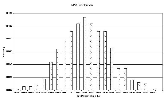
Figure 1
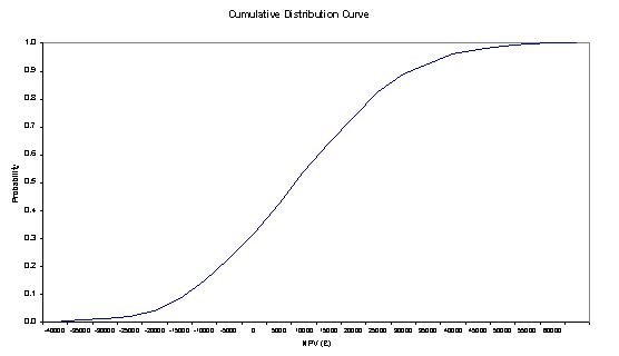
Figure 2
Once the model is running it is important that a process of validation is undertaken to ensure that it is working as intended. This needs to be nothing more than checking that the results are comparable to those shown in the Results Table.
Having confirmed that the model is working correctly students should be encouraged to analyse the results. This could involve answering questions such as those set out below:
Important though it is to get students using the risk simulation model and analysing the results, this is really only the beginning. One of the biggest benefits to be gained from using a risk simulation model without the aid of add-in packages like @Risk is the scope for further model development.
Modifications to the model could take the form of modifications to both the macro and the spreadsheet model. Changes to the macro that could be explored include aspects such as increasing the number of simulations carried out. 500 simulations were used in this instance but it is a simple matter to increase this to 2,000 or 5,000.
Changes to the model could include the incorporation of some of the following:
Various versions of this application have been used on a variety of Managerial Economics and Business Strategy modules at both undergraduate and postgraduate levels. Students have not been Economics majors rather they have been Business Studies majors or DMS/MBA students. During the course of their managerial careers such students will encounter investment projects. An understanding of risk analysis in general and risk simulation in particular is likely to be very useful. Although a self-constructed risk simulation, such as the one presented in this instance, has limitations compared to those developed using the resources of an add-in package like @Risk, this is offset by the depth of understanding of risk simulation and associated concepts gained by business and management students.
Barlow, T. F. (1999) Excel Models for Business and Operations Management, John Wiley and Sons, Chichester.
Bridge, J (1989) Managerial Decisions with the Microcomputer, Prentice Hall, Hemel Hempstead.
Judge, G. (1999) 'Simple Monte Carlo studies on a spreadsheet' CHEER, Vol 13, No 2, pp 12-14.
Oakshott, L. (1997) Business Modelling and Simulation, Pitman.