Volume 13, Issue 2, 1999
The Heckscher-Ohlin Model with variable input coefficients in spreadsheets
- J. Wilson Mixon, Jr. and Soumaya M. Tohamy
- Berry College, Campbell School of Business
Abstract
This paper describes the presentation of the Heckscher-Ohlin model of international trade using an Excel workbook. The model consists of a two-factor economy producing two goods. The production of each is represented by a Cobb-Douglas production function. Given the fixed supplies of the two resources, labour and land, the model demonstrates how competitive markets allocate the resources between two competing uses, cloth production and food production. Presenting this model with Excel allows instructors to illustrate production functions, the derivation of the production possibilities frontier, and the effect of prices on resource allocation, inter alia. It also allows the illustration of the effects of changes in technology, factor supplies, or product prices on economic outcomes. Perhaps more importantly, the use of Excel allows students access to a "live" study guide, within which they can replicate and extend analysis presented by the instructor. This provides a deeper understanding of the theory. At the same time, the students are becoming more familiar with the use of spreadsheets, developing a skill that will serve them well throughout their lives.
1. Introduction
Liberal education's purpose is not to teach immediately applicable skills. This does not mean, however, that those teaching courses like economics should shun technical advances. Doing so is a disservice to our students for two reasons. First, and most immediately, technical advances can make us better instructors, as we use these techniques to provide students with a deeper understanding of content material. Second, even though the purpose of a course like economics is not to train, training does have immediate value. Wight (1999) notes that more than seventy percent of economics majors seek employment upon graduation rather than attending graduate studies, and he concludes that the "Economics faculty have a moral obligation to address the legitimate employment concerns of these students" (page 22).
Paetow (1998) identifies a major advantage of integrating the computer into the classroom: “Modern computer technology has expanded the range of complexity and sophistication in economic research and teaching alike”. In particular, he shows how Excel can be used to advantage. Excel rivals more specialized software in terms of its ability to analyze and depict complex relationships. Its use offers unique advantages. It is easily integrated into the Microsoft Suite, especially with PowerPoint, allowing for effective presentations. Because this suite, or very similar ones, is so widely used in private and public agencies, having students use Excel provides a way for them to learn a useful tool as they develop their knowledge of the content.
This paper uses Excel to develop a central component of the analysis of international trade, the Heckscher-Ohlin Model. This is an especially useful model to develop because it combines and demonstrates the interrelatedness of so many tools of the economist: isoquants, expansion paths, the Edgeworth box diagram, and the production possibilities curve.
The paper proceeds as follows. Section 2 develops the model. It shows the pertinent economic relationships, based on specific functional forms. Then Section 3 shows the most important of the relationships in graphical form, with all graphs being from an Excel workbook.
2. The Model
We use the Cobb-Douglas production functions:
(1) C = ALCaTC1-a
and
(1’) F = BLFbTF1-b,
where C(F) is the quantity of clothing (food) being produced, LC(LF) is the quantity of labour employed in cloth (food) production, and TC(TF) is the quantity of land employed in cloth (food) production. The coefficient A(B) is a positive constant reflecting technology.
First, define the unit isoquants, showing the amount of land used given the employment of labour in producing each unit of cloth (food). These are:
(2) TC = [A-1LC-a]1/(1-a)
and
(2’) TF = [B-1LF-b]1/(1-b) .(1)
The first-order conditions, coupled with linear homogeneity, allow the derivation of lines that show factor price ratios that are consistent with various input combinations. Following Krugman and Obstfeld, these are denoted as CC and FF respectively. The equation for the line CC (the cloth industry's expansion path) is:
(3) r = (1/a-1)(LC/TC)w ,
where w is the wage rate (payment per unit of labour) and r is the rental rate (per unit of land). The corresponding FF line, similarly defined, is:
(3’) r = (1/b-1)(LF/TF)w.
So far, the model transforms the expansion paths in the two industries into equations involving factor prices in each of the two industries. To move closer to closing the model requires that product prices be related to the information above. This is accomplished by imposing equilibrium conditions for competitive markets, that price equals marginal cost (MC) in each industry. Since MC = w/MPL in each industry, this imposition implies the following:
(4) PC = w(Aa)-1(1/a-1)a-1(w/r)a-1
and
(4’) PF = w(Bb)-1(1/b-1)b-1(w/r)b-1.
These two equations provide this critical relationship between the ratio of input prices and that of product prices:
(5) (w/r) = [Aa(1/a-1)1-a(Bb-1)-1(1/b-1)b-1(PC/PF)]1/(a-b).
Determining how much labour and land are used in each of the two industries can now close the model. The expansion paths give the key to this determination.
(6) TC = (w/r)(1/(a-1))LC
and
(6’) TF = (w/r)(1/(b-1))LF.
But, LF = L-LC and TF = T-TC.

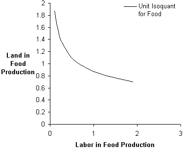
Figure 1: Unit Isoquant for Food.
Appropriate substitution allows TC and TF to be stated as a linear function of LC. The resulting equations are:
(7) TC = kLC
and
(7') TF = mL-mLC
where k=(w/r)(1-a)/a and m = (w/r)(1-b)/b.
The equations above represent a closed system for a competitive two-sector small-country economy. This system can be represented graphically within Excel. The next section provides an overview of this representation. It does so by representing equations (2), (3), and (5), along with (7) and (7') as a set.
3. What Students See: Graphical Representation
The graphical representation of the model begins with the "unit" isoquant, showing the many input combinations that can result in a single unit of output (see Figure 1). The unit isoquant for one of the two goods, food, is shown. Typically students will have learned the fixed-coefficient, single-input Ricardian model at this point. The graph allows for a generalization and a discussion of the concept of substitution.

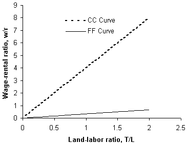
Figure 2: Factor Prices and Input Choice.

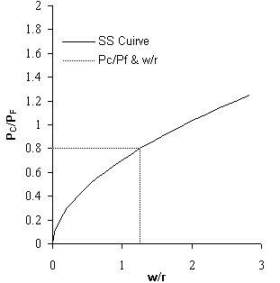
Figure 3: Factor Prices and Goods Prices.
The next logical step is to determine the input ratios for each of the two goods depicted by the model. Based on the usual assumption of constant return to scale production functions, we can show students that in each of the two industries, the land/labour ratio is uniquely related to the wage/rental ratios. Figure 2 presents the relationships for the Cobb-Douglas functions used.
The inquisitive student can see the puzzle coming together. Figure 2 raises as many questions as it answers. Specifically, it makes obvious that two questions must be addressed before the system can be closed: What (w/r) will prevail? And how do the two industry-specific land-to-labour ratios add up to the economy-wide quantities of land and labour? (As a later graph makes clear, the Heckscher-Ohlin model relies on the assumption that land and labour quantities do not depend on the wage-rental ratio. That is, the economy-wide supply curves for both labour and land are vertical.)
First, the wage-rental ratio is determined. This is accomplished by developing the unique relationship between (w/r) and the relative prices of the two goods, PC/PF. The relative price of goods is exogenous, determined by world markets (this development is for the small-country case; it can be extended to make the prices of the goods endogenous). Once PC/PF is determined, so are (w/r) (in Figure 3) and the land-labour ratio in each of the two sectors. What remains is to determine the level of employment of each input in each of the two sectors.

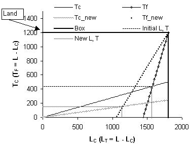
Figure 4: Effects of Changed Prices.
Figure 4 shows how the model is closed. It shows the employment level of labour and land in each of the two sectors. The graph shows these employment levels at each of two sets of product prices. The Excel workbook also shows the effects of changed levels of land and labour. The bold line that defines the origin for food production is labeled E_box for Edgeworth box. Excel does not allow showing the actual number of units of labour and land in food production, but these quantities are easily determined. Furthermore, the spreadsheet on which the graph below is located provides the employment levels and the associated output levels.
Other sheets in the workbook allow the student to change land and labour and to determine the effects of these changes on the equilibrium values.
4. Summary
Excel provides a powerful and flexible tool for letting students learn by doing. This paper has shown how one of the more complex models encountered by students, the Heckscher-Ohlin model, can be represented in an Excel workbook. The workbook lets students change parameters of the production functions, product prices, and resource endowments. In doing so, they can examine the comparative statics of the system while becoming more aware of how to use Excel as a tool to develop models and present information.
The authors may be contacted at: Campbell School of Business, Berry College, Mount Berry, GA 30149-5024. E-mail: wmixon@campbell.berry.edu .
References
Paul R. Krugman and Maurice Obstfeld. 1997. International Economics: Theory and Practice, 4th edition. New York: Harper Collins.
Holger Paetow. 1998. “Long-Run Dynamic Market Equilibrium Simulation Through the Use of Spreadsheets.” Computers in Higher Education Economics Review.
Jonathan B. Wight, 1999. Using Electronic Data Tools in Writing Assignments. Journal of Economic Education. Vol. 30, No. 1, winter 1999, 21-27.
(1) This is just one way in which the model could be illustrated. We use it
following the presentation in Krugman and Obstfeld (1997).
|
What's Related: · Other articles on the use of spreadsheets in teaching economics |

