Volume 13, Issue 1, 1999
Explaining Input-Output and Equilibrium Relationships Using Excel Display Facilities
- David Whigham and Jeanie Whyte
- Glasgow Caledonian University
Introduction
The background to this work was the need to provide an efficient visual representation of inter and intra industry economic flows for a research student who was to be employed in a funded project to develop a set of National Accounts for Scotland - the Caledonian Blue Book 1997. Since one of the eventual objectives of the project would involve the generation and use of input-output tables, it was decided to develop a simple model of an economic system that would thereby display the relationships more overtly than would conventional matrix methods. It was intended that this visual model would then lay the foundations for a more intuitive understanding of the matrix procedures that would inevitably have to be employed in more realistic applications1. Thereafter, it became clear that the models developed could be of considerable use for teaching purposes.
In short, the generated models provide an introductory visual guide to the intricacies of input - output analysis and allow experimentation and investigation of the models’ respective properties to be carried out by the user in an overtly interactive way. Full versions of the models are obtainable free of charge by contacting the authors.
The simple model
In the first model, the system of economic relations is very simple. Two primary products, Coal (C) and Iron (I), are used to produce a final consumption good, Steel (S), that provides the means of survival for all employed economic agents. The latter include Coal, Iron and Steel workers (CW, IW and SW) who require to be provided with a proportion of the final output of Steel (S to CW, S to IW and S to SW) in order to supply their labour. It is also assumed that the production of Coal and Iron requires Steel (S to C and S to I) and that production of Steel itself also requires some Steel (S to S).
The ‘hub’ of the system, however, is the total initial demand for Steel that is exercised by the owners of the property from which Coal and Iron are derived, i.e. Coal mine owners (CMO) and Iron mine owners (IMO). These rental demands (S to CMO and S to IMO) must be satisfied if any economic activity is to take place.
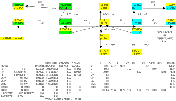
The structure of this basic model is contained in Model 1 and shown in Figure 1.
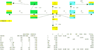
Figure 1
Click above to download image
It is suggested that users should employ the model in the following way.
The output of Steel required by the two groups of owners (20 in the illustration) should be entered as a starting value to the cell labelled S. Once this has been done the implied resource requirements of the system are transmitted as shown. Given the parameter values in the un-shaded cells it is now an easy matter to trace through the system and observe the effects of any initial value for the amount of Steel required by the owners. Thus, since each unit of Steel requires 2 units of Coal (c/s), 20 units gives a required Coal output of 40. Each unit of Coal, however, requires 0.05 Coal workers (cw/c) so a total of 2 Coal workers are needed. In turn, each of these Coal workers needs 0.1 units of Steel (s/cw) for final consumption purposes and so an additional demand for 0.2 units of Steel is generated as indicated in the top left hand shaded cell in the diagram.
However, since the ultimate task is to determine the total amount of Steel that must be produced, cell labelled S NEEDED has been used to contain the sum of all the requirements that have been generated by the initial attempt to supply the 20 units demanded by the mine owners. This is obtained from:
S to CMO + S to IMO + S to CW + S to IW + S to SW + S to C + S to I + S to S
As is clear from the illustration the total system requirements (36) exceed the 20 units produced, and so the system is not in balance.
These real flows have been translated into corresponding financial flows in the lower left hand section of Figure 1, where the price of Steel (PS) has been set at an arbitrary value.
Formulae were written to compute the rents, wages and prices required to supply each group of agents with exactly sufficient income to purchase the amounts of Steel that they require. For example, in order for the Iron mine owners to purchase their required 10 units of Steel at a steel price (PS) = 10, the payment to the owners (RIMO) must equal 100 currency units. Thus, the appropriate entry would be PS times (S to IMO). Similar logic applies to the rents, wages and prices obtained by the other groups - except for the price of Steel. This is because the system has one degree of freedom, and so the price of Steel in this model is an arbitrary numeraire (set to a value of 10 in the illustration). This is easily confirmed by allowing the price of Steel to change, whereupon all the other prices, wages and rents will adjust proportionally after calculation.
Clearly since the real flows of the system are not in balance, neither are the financial flows and this is indicated by the fact that the real deficit of Steel (-16 units) has been translated to a financial deficit for Steel producers of -160 (i.e. -16 times the (arbitrary) price of Steel).
Finally, the right hand section of Figure 1 shows the complete set of disaggregated financial flows associated with the current disequilibrium situation, where any individual entry is the financial expenditure paid by the row element to the associated column element. Thus, producers of Coal spend 80 currency units on Steel, 2 currency units on Coal workers and 100 currency units on rent to Coal mine owners.
This model can now be used to resolve for the equilibrium amount of Steel to be produced.
This is easily done by replacing the value of 20 that is currently being used for the cell labelled S with the formula: =SREQU, where the cell, B23, containing the total required amount of Steel (currently 36 units) has been named as SREQU. Entering this formula ensures that the output of Steel must equal the sum of all demands for Steel generated by the initial amount of Steel that has to be produced.
When this entry is made, with the default settings, Excel will usually return the error message “cannot resolve circular references”, and a value of zero will be returned. This clearly shows the circular nature of the flows that have been generated. By this it is meant that since production of Steel requires some Steel itself, the eventual output of Steel including the amount for its own needs cannot be computed until the amount of Steel required is itself known.
However, it is an easy matter to force Excel to resolve this circular argument. To do this, select: Tools, Options, Calculation and then check the iteration box. When OK is clicked, the model will iterate a default 100 times and will eventually settle down at the equilibrium value of S. The flashing values that appear in all calculated cells after Calc (F9) has been pressed give a dynamic demonstration of the iterative procedure that is taking place.
The eventual equilibrium value for S with the given parameters is contained in Model 2 and shown in Figure 2, where it is also clear that the financial flows for each of the groups are now in balance. Clearly the model has not only determined the required output of Steel, and the associated outputs and employment of the primary inputs and workers, but also the prices, wages and rents necessary to allow the required amounts of Steel to be purchased. The value added at each stage of the production process have also been added to the generated accounts.
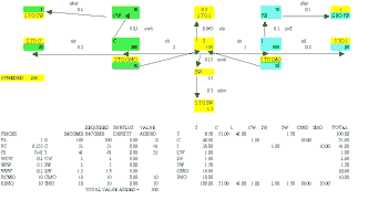
Figure 2
Click above to download image
Investigating Change
At this stage it is suggested that time is spent investigating the effects of changes in the parameter values of the system. This is because a number of important implications can easily be derived. The following are some suggestions.
(a) Increase the amount of Coal needed for each unit of Steel (c/s) from 2 to 2.5. The amount of Steel produced will increase but the absolute prices of both Coal and Iron will decline. This however, is done in such a way that the price of Coal relative to the price of Iron increases.
Now restore the amount of Coal needed for each unit of Steel to its original value of 2.
(b) Increase the number of Coal workers required per unit of Coal (cw/c) from 0.05 to 0.1. The amount of Steel produced increases, the absolute price of Coal increases and the absolute price of Iron decreases. Consequently, the price of Coal relative to Iron must increase. It should also be noted that the wages of Coal workers are unchanged although the income that they receive increases by dint of the need to employ more of them.
Now restore the number of Coal workers needed for each unit of Coal to its original value of 0.05.
(c) Suppose that the amount of Steel required by each Coal worker (s/cw) increases from 0.1 to 0.15. The amount of Steel required will increase, the absolute price of Coal will increase and the absolute price of Iron will decrease. Consequently, the price of Coal relative to the price of Iron will increase. Importantly, however, not only are there more Coal workers employed, but their wage rate has also increased, while the wage rates of the other groups of workers remain unchanged.
Now restore the amount of Steel required by each Coal worker to its original value of 0.1.
(d) Suppose that the amount of Steel required by the owners of Coal (S to CMO) falls from 10 to 5, while the amount of Steel required by the owners of Iron (S to IMO) increases from 10 to 15. Now, although the total amount of Steel required by both groups of owners has not changed, the relative distribution of this total has moved in favour of the owners of Iron.
As would be expected, the total amount of Steel produced by the system remains unchanged in such circumstances, but this is not true for the prices of Coal and Iron, nor for the rents paid to the owners. To be exact, the absolute price of Coal decreases and the absolute price of Iron increases, with the result that the price of Coal relative to the price of Iron decreases.
Also, the rents payable to the owners of Coal and Iron decrease and increase respectively. These price and rent changes are entirely understandable when it is noted that by requiring less Steel the owners of Coal reduce the costs that the producers of Coal must endure, thereby allowing an absolute reduction in the price of Coal.
Now restore the amounts of Steel required by the owners of Coal and Iron to their original values of 10 and 10 respectively.
(e) It is an easy matter to ‘break’ the model in the sense that the generated demands of the system are impossible to satisfy. For example, increase the amount of Coal required by each unit of Steel (c/s) from 2 to 3, and it will be found that the iteration process cannot find a finite solution. This is because the necessary amount of Steel now required to supply the Coal industry cannot be generated by the Steel industry at its current level of technical efficiency.
Extending the Model
It is, of course the case, that a realistic model would require the inclusion of many more primary, intermediate and final products, and it is simply not practical to adopt the current approach in such circumstances - a conventional matrix approach would be required.
Nevertheless, it should be emphasised that the purpose of the outlined model is to provide a firm, easily observed platform from which realistic extensions could be considered by matrix techniques.
This said, there are further extensions of the current model that can prove instructive without making the models too cumbersome.
Model Extension 1
The first of these is to suppose that Coal, Iron and Steel each require distribution to the ultimate users, i.e. Coal distribution (CD), Iron distribution (ID), and Steel distribution (SD). Also assume that this will require Steel itself (S to CD, S to ID and S to SD), as well as Coal, Iron and Steel distribution workers (CDW, IDW and SDW) who in turn require Steel as payment for their services (S to CDW, S to IDW and S to SDW).
This extension of the model is contained in Model 3 and shown in Figure 3 where it is assumed that the end user pays for the distribution of the inputs and the final products.
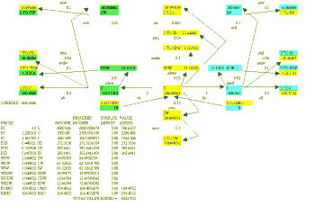
Figure 3
Click above to download image
Once again the generated flows are easily observed and the required equilibrium prices and wage rates now include the prices of distributing Coal, Iron and Steel as well as the wage rates that are to be paid for the services of Coal, Iron and Steel distribution workers. The value added at each stage is also computed.
As with the simple model, the extended version is easily subjected to investigation of the effects of parameter variations, although in this case, because of the more complex nature of the circular relations generated it would be necessary to change the Excel calculation mode from automatic to manual.
Model Extension 2
The second extension of the model is to introduce a third essential input (Chemicals - N) to the Steel production process. This is done in such a way however, that Chemicals can only be produced by a second country - B, which cannot produce Iron. Thus country A produces Coal, Iron and Steel and imports Chemicals from country B, while Country B produces Coal Chemicals and Steel and must import its Iron requirements from Country A.
To investigate the properties of this two country model, it is assumed in the first instance, that the conditions of production are ‘symmetrical’ for both Iron and Chemicals. In other words, each unit of Steel production in A uses the same amount of Chemicals as each unit of Steel production in B needs of Iron. Equivalently, each unit of Steel in B requires the same amount of Iron as each unit of Steel in A needs of Chemicals.
These symmetry assumptions ensure that the economies of the two countries are effectively images of each other, with the major effect being that Iron production in A must now not only satisfy the Iron requirements of its own Steel industry, but also those from the Steel industry in country B. Conversely, the Chemicals industry in B must now satisfy the requirements of country B’s steel industry, as well as those of its own.
When these added circular relations, as well as the initial set of assumed productive relations, are added to the model, the system will settle down to an equilibrium situation in which production of Steel is the same in each country. Furthermore, as Model 4 can be used to demonstrate, the numeraires are seen to be equal in this special case.
However, if the amount of Chemicals required per unit of steel in country A were to exceed the amount of iron required per unit of Steel in country B then a reallocation will be required. This is easily confirmed by making the appropriate change to Model 4, whereupon it will be found that steel production in B must increase relative to steel production in B. For example, with each unit of Steel in A requiring 0.2 units of Chemicals, and each unit of Steel in B requiring only 0.1 units of Iron, then the equilibrium level of steel production will require that B produces more Steel than A.
More importantly however, it will also be found that with equal numeraires in each country, the financial balances will no longer all be zero. To be exact, country B will now run a financial surplus while country B will run a financial deficit.
This stems entirely from the fact that even with the same numeraire the internal prices of Iron in A and Chemicals in B are no longer equal (as a result of each unit of steel production in A now requiring more chemicals from B than Steel production in B requires form A’s Iron industry. The net effect is clearly to generate a trade imbalance between the two countries as long as the numeraires remain identical.
However, it is an easy matter to get the model to recompute one or other of the numeraires so that the trade imbalance is eliminated. This can be done by employing the Solver to find the value of the numeraire in one of the countries that eliminates the surpluses and deficits from the financial balances in both partners. The Solver settings are included in Model B and need never be changed.
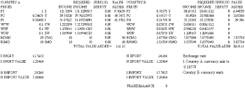
When this is done it should be clear that what has really been computed is the exchange rate between the numeraires in each of the countries. Thus for example, if country A’s numeraire is set at 1 and if each unit of output in its steel industry still requires more chemicals than in B, the numeraire in country B will be computed at a value of less than 1 - implying a devaluation of country A’s currency vis a vis country B, and having the effect of removing the trade imbalance. When used with the values suggested above (Chemicals per unit of Steel in A = 0.2; Iron per unit of Steel in B = 0.1 then the effects are calculated by Model 4 and indicated in Figure 4.
Model Extension 3
The final extension of interest is to assume that there is a work force of given size. Suppose, for example, that the equilibrium requirement for all types of workers is less than the available work force. Also suppose that the state decides to give each of these unemployed workers ub units of steel, where ub is normally less than the amount paid to employed workers. These benefits to the unemployed are obtained by a uniform rate of taxation on the output of the Steel industry.
The effects of such a regime are contained in Model 5 and shown in Figure 5.
This model can be used to show that if ub = 0, then (with the given parameters) the equilibrium production level of Steel is 100 units, and 10 workers out of the work force of 45 are unemployed. If, however, ub is increased to 0.05 units of Steel then the need to supply this extra Steel causes the number of unemployed workers to decline to 9.2, and the output of Steel to increase to 102.3 units.
A comparative model
The relations considered in Model 2 have been reconstituted into a version that allows any two ‘before and after’ sets of production parameters to be compared directly in both numerical and graphical forms. This comparative model is contained in Model 6 and allows endless investigation of the effects of changes in the conditions of production to be observed.
Conclusions
This discussion and the models presented have attempted to provide a clear visual display of what are by no means trivial inter - relationships in a simple economic system. It is to be hoped that the key feature of these interactions - their circularity - is readily appreciated as a result of Excel’s ability to display the constituent parts of the model in considerable detail and to give clear indications of the iterative procedures that have to be employed in order to resolve the circularities.
Note: The authors may be contacted by e-mail to d.whigham@gcal.ac.uk
References
Gibson H., Riddington G., Whigham D. and Whyte, J., Caledonian Blue Book - National Accounts for Scotland 1951-96. Glasgow Caledonian University 1997.
Judge G. Quantitative Analysis for Economics and Business. Harvester Wheatsheaf 1990.
Sraffa P. Production of Commodities by Means of Commodities. Cambridge: Cambridge University Press, 1960.
Whigham D. Quantitative Business Methods Using Excel 5.0. Oxford University Press, 1998.
Notes
(1) For an excellent introduction to input-output analysis using matrix techniques on a spreadsheet see Judge, 1990.
|
What's Related: · Other articles on the use of spreadsheets in teaching economics |


